# Load the pandas libraryimport pandas as pd# Load numpy for array manipulationimport numpy as np# Load seaborn plotting libraryimport seaborn as snsimport matplotlib.pyplot as plt# Set font sizes in plotssns.set(font_scale =2)# Display all columnspd.set_option('display.max_columns', None)# Import income2 dataincome = pd.read_csv("../data/Income2.csv", index_col =0 )income
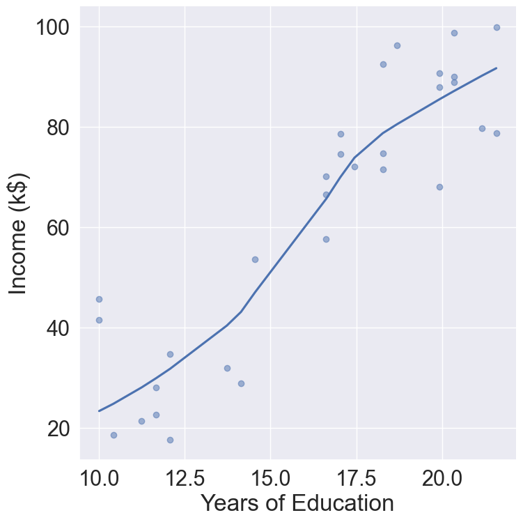
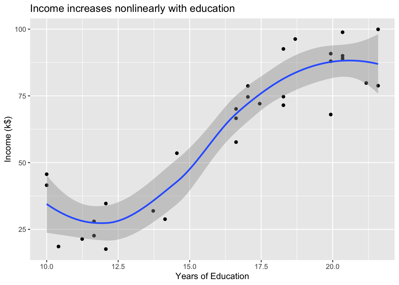
# Plot income ~ Educationincome %>%ggplot(mapping =aes(x = Education, y = Income)) +geom_point() +geom_smooth() +labs(title ="Income increases nonlinearly with education",x ="Years of Education",y ="Income (k$)")
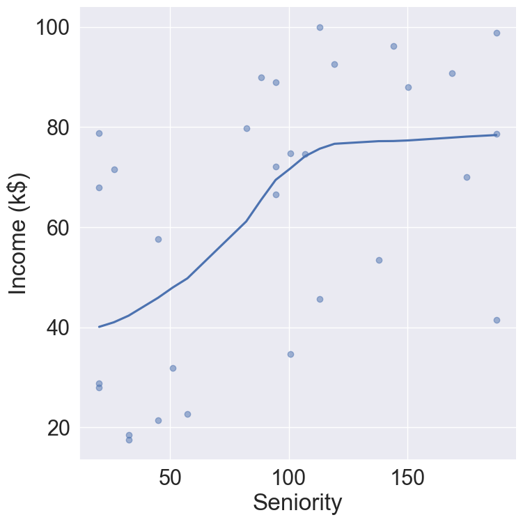
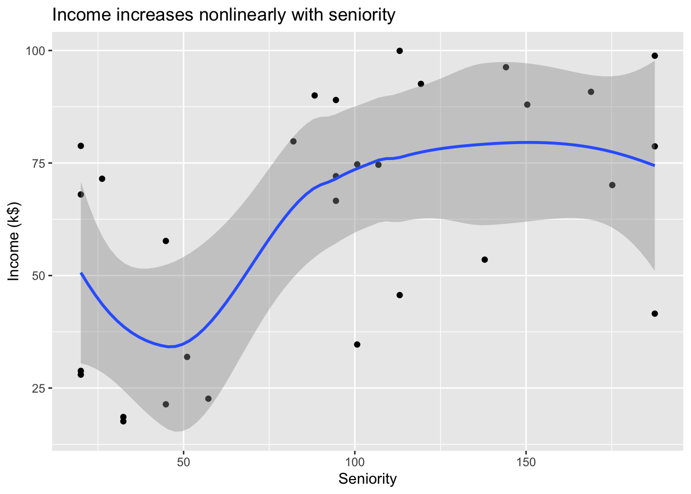
# Plot income ~ Seniorityincome %>%ggplot(mapping =aes(x = Seniority, y = Income)) +geom_point() +geom_smooth() +labs(title ="Income increases nonlinearly with seniority",x ="Seniority",y ="Income (k$)")
Can we predict Income using Years of Education? Can we predict Income using Seniority? Perhaps we can do better with a model using both? \[
\text{Income} \approx f(\text{Education}, \text{Seniority})
\]
\(Y\): Income is the response, or target, or output, or outcome, or dependent variables that we wish to predict.
\(X\): Education and Seniority. \[
X = \begin{pmatrix} X_1 \\ \vdots \\ X_p \end{pmatrix}
\] is the vector of features, or inputs, or predictors, or independent variables.
We assume the model \[
Y = f(X) + \epsilon,
\tag{1}\] where
\(f\) represents the systematic information that \(X\) provides about \(Y\);
The error term\(\epsilon\) captures measurement errors and other discrepancies.
In essence, statistical learning refers to a set of approaches for estimating the function \(f\).
1.2 Why estimate \(f\)?
Prediction. With a good estimate \(\hat f\), we can predict \(Y\) at new points \[
\hat Y = \hat f (X).
\]
Inference.
We can understand which components of \(X=(X_1, \ldots, X_p)\) are important in explaining \(Y\), and which are irrelevant. For example, Seniority and Years of Education have a big impact on Income, but Marital Status typically does not.
Depending on the complexity of \(f\), we may be able to understand how each component \(X_j\) of \(X\) affects \(Y\). For example, how much extra income will one earn with two more year of education? Does a linear relationship hold?
Causal inference. We may infer whether purposedly changing the values of certain predictors will change outcomes. For example, does an advertising campaign increase the sales? Or it’s just seasonal change in sales?
1.3 The optimal (but unrealistic) \(f\)
It can be shown (HW1) that \[
f_{\text{opt}} = \operatorname{E}(Y | X)
\] minimizes the mean-squared prediction error \[
\operatorname{E}[Y - f(X)]^2,
\] where the expectations averages over variations in both \(X\) and \(Y\).
However we almost never know the conditional distribution of \(Y\) given \(X\). In practice, we use various learning methods to estimate \(f\).
Statistical learning techniques may yield better \(\hat f\), thus decreasing the reducible errors.
Even if we knew the truth \(f\), we would still make errors in prediction due to the irreducible error.
1.5 How to estimate \(f\)?
Our goal is to apply a statistical learning method to find a function \(\hat f\) such that \(Y \approx \hat f(X)\).
1.5.1 Parametric or structured model
Step 1. We make an assumption about the functional form, or shape, of \(f\).
For example, one may assume that \(f\) is linear in \(X\): \[
f(X) = \beta_0 + \beta_1 X_1 + \cdots \beta_p X_p.
\]
Step 2. We use the training data \(\{(x_1, y_1), \ldots, (x_n, y_n)\}\) to train or fit the model.
The most common approach for fitting the linear model is least squares. However there are many other possible ways to fit the linear model (to be discussed later).
Blue surface is the true \(f\)
Yellow surface is the linear model fit \(\hat f\)
Figure 3: Linear approximation of \(f\).
Although it is almost never correct, a linear model often serves as a good and interpretable approximation to the unknown true function \(f\).
1.5.2 Non-parametric model
Non-parametric methods do not make explicit assumptions about the functional form of \(f\). Instead they seek an estimate of \(f\) that gets as close to the data points as much as possible without being too rough or wiggly.
Advantages: better fit.
Disadvantage: many more paremeters; need more training samples to accurately estimate \(f\).
Thin-plate spline (discussed later) approximates the true \(f\) better than the linear model.
Blue surface is the true \(f\)
Yellow surface is the thin-plate spline fit \(\hat f\)
Figure 4: Thin-plate spline fit of \(f\).
We may even fit an extremely flexible spline model such that the fitted model makes no errors on the training data! By doing this, we are in the danger of overfitting. Overfit models do not generalize well, which means the prediction accuracy on a separate test data can be very bad.
Blue surface is the true \(f\)
Overfitting
Figure 5: Overfitting of \(f\).
1.6 Some trade-offs
Prediction accuracy vs interpretability.
Linear models are easy to interpret; thin-plate splines are not.
Good fit vs over-fit or under-fit.
How do we know when the fit is just right?
Parsimony vs black-box.
Practitioners often prefer a simpler model involving fewer variables over a black-box predictor involving them all.
Figure 6: Trade-off of model flexibility vs interpretability.
1.7 Assessing model accuracy
Given training data \(\{(x_1, y_1), \ldots, (x_n, y_n)\}\), we fit a model \(\hat f\). We can evaluate the model accuracy on the training data by the mean squared error\[
\operatorname{MSE}_{\text{train}} = \frac 1n \sum_{i=1}^n [y_i - \hat f(x_i)]^2.
\] The smaller \(\operatorname{MSE}_{\text{train}}\), the better model fit.
However, in most situations, we are not interested in the training MSE. Rather, we are interested in the accuracy of the predictions on previously unseen test data.
If we have a separate test set with both predictors and outcomes. Then the task is easy, we choose the learning method that yields the best test MSE \[
\operatorname{MSE}_{\text{test}} = \frac{1}{n_{\text{test}}} \sum_{i=1}^{n_{\text{test}}} [y_i - \hat f(x_i)]^2.
\]
In many applications, we don’t have a separate test set. Is this a good idea to choose the learning method with smallest training MSE?
Figure 7: Black curve is truth. Red curve on right is the test MSE, grey curve is the training MSE. Orange, blue and green curves/squares correspond to fits of different flexibility.
Figure 8: Here the truth is smoother, so the smoother fit and linear model do really well.
Figure 9: Here the truth is wiggly and the noise is low, so the more flexible fits do the best.
As the previous three examples illustrate, the flexibility level corresponding to the model with the minimal test MSE can vary considerably among data sets.
Later we will discuss the cross-validation strategy to estimate test MSE using only the training data.
1.8 Bias-variance trade-off
The U-shaped observed in the test MSE curves (Figure 7-Figure 9) reflects the bias-variance trade-off.
Let \((x_0, y_0)\) be a test observation. Under the model Equation 1, the expected prediction error (EPE) at \(x_0\), or the test error, or generalization error, can be decomposed as (HW1) \[
\operatorname{E}[y_0 - \hat f(x_0)]^2 = \underbrace{\operatorname{Var}(\hat f(x_0)) + [\operatorname{Bias}(\hat f(x_0))]^2}_{\text{MSE of } \hat f(x_0) \text{ for estimating } f(x_0)} + \underbrace{\operatorname{Var}(\epsilon)}_{\text{irreducible}},
\] where
the expectation averages over the variability in \(y_0\) and \(\hat f\) (function of training data).
Typically as the flexibility of \(\hat f\) increases, its variance increases and its bias decreases.
Figure 10: Bias-variance trade-off.
1.9 Classical regime vs modern regime
Above U-shaped test MSE curves are in the so-called classical regime where the number of features (or the degree of freedom) is less than the training samples.
In the modern regime, where the number of features (or the degree of freedom) can be order of magnitude larger than the training samples (recall that ChatGPT3 model has 175 billion parameters!), the double descent phenomenon is observed and being actively studied. See the recent paper and references therein.
When the outcome \(Y\) is discrete, for example, email is one of \(\mathcal{C}=\){spam, ham} (ham=good email), handwritten digit is one of \(\mathcal{C} = \{0,1,\ldots,9\}\).
Our goals are to
build a classifier \(f(X)\) that assigns a class label from \(\mathcal{C}\) to a future unlabeled observation \(X\);
assess the uncertainty in each classification;
understand the roles of the different predictors among \(X=(X_1,\ldots,X_p)\).
To evaluate the performance of classification algorithms, the training error rate is \[
\frac 1n \sum_{i=1}^n I(y_i \ne \hat y_i),
\] where \(\hat y_i = \hat f(x_i)\) is the predicted class label for the \(i\)th observation using \(\hat f\).
As in the regression setting, we are most interested in the test error rate associated with a set of test observations \[
\frac{1}{n_{\text{test}}} \sum_{i=1}^{n_{\text{test}}} I(y_i \ne \hat y_i).
\]
Suppose \(\mathcal{C}=\{1,2,\ldots,K\}\), the Bayes classifier assigns a test observation with predictor vector \(x_0\) to the class \(j \in \mathcal{C}\) for which \[
\operatorname{Pr}(Y=j \mid X = x_0)
\] is largest.
In a two-class problem \(K=2\), the Bayes classifier assigns a test case to class 1 if \(\operatorname{Pr}(Y=1 \mid X = x_0) > 0.5\), and to class 2 otherwise.
The Bayes classifier produces the lowest possible test error rate, called the Bayes error rate\[
1 - \max_j \operatorname{Pr}(Y=j \mid X = x_0)
\] at \(X=x_0\). The overall Bayes error is given by \[
1 - \operatorname{E} [\max_j \operatorname{Pr}(Y=j \mid X)],
\] where the expectation averages over all possible values of \(X\).
Unfortunately, for real data, we don’t know the conditional distribution of \(Y\) given \(X\), and computing the Bayes classifier is impossible.
Various learning algorithms attempt to estimate the conditional distribution of \(Y\) given \(X\), and then classify a given observation to the class with the highest estimated probability.
One simple classifier is the \(K\)-nearest neighbor (KNN) classifier. Given a positive integer \(K\) and a test observation \(x_0\), the KNN classifier first identifies the \(K\) points in the training data that are closest to \(x_0\), represented by \(\mathcal{N}_0\). It then estimates the conditional probability by \[
\operatorname{Pr}(Y=j \mid X = x_0) = \frac{1}{K} \sum_{i \in \mathcal{N}_0} I(y_i = j)
\] and then classifies the test observation \(x_0\) to the class with the largest probability.
Figure 12: Black curve is the KNN decision boundary using \(K=10\). The purple dashed line is the Bayes decision boundary.
Smaller \(K\) yields more flexible classification rule.
Figure 13: Left panel: KNN with \(K=1\). Right panel: KNN with \(K=100\).
Bias-variance trade-off of KNN.
Figure 14: KNN with \(K \approx 10\) achieves the Bayes error rate (black dashed line).