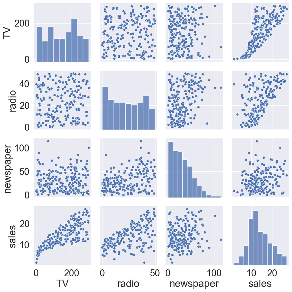
# Load the pandas libraryimport pandas as pd# Load numpy for array manipulationimport numpy as np# Load seaborn plotting libraryimport seaborn as snsimport matplotlib.pyplot as plt# Set font sizes in plotssns.set(font_scale =2)# Display all columnspd.set_option('display.max_columns', None)# Import Advertising dataAdvertising = pd.read_csv("../data/Advertising.csv", index_col =0)Advertising
Is there a relationship between advertising budget and sales?
How strong is the relationship between advertising budget and sales?
Which media contribute to sales?
How accurately can we predict future sales?
Is the relationship linear?
Is there synergy among the advertising media?
3 Simple linear regression vs multiple linear regression
In simple linear regression, we assume a model \[
Y = \underbrace{\beta_0}_{\text{intercept}} + \underbrace{\beta_1}_{\text{slope}} X + \epsilon.
\] For example \[
\text{sale} \approx \beta_0 + \beta_1 \times \text{TV}.
\] The lower left plot in the pair plot (R) displays the fitted line \[
\hat y = \hat \beta_0 + \hat \beta_1 \times \text{TV}.
\]
In multiple linear regression, we assume the model \[
Y = \beta_0 + \beta_1 X_1 + \beta_2 X_2 + \cdots + \beta_p X_p + \epsilon.
\] For example, \[
\text{sales} \approx \beta_0 + \beta_1 \times \text{TV} + \beta_2 \times \text{radio} + \cdots + \beta_3 \times \text{newspaper}.
\] We review the multiple linear regression below.
4 Estimation in multiple linear regression
We estimate regression coefficients \(\beta_0, \beta_1, \ldots, \beta_p\) by the method of least squares, which minimizes the sum of squared residuals \[
\text{RSS} = \sum_{i=1}^n (y_i - \hat y_i)^2 = \sum_{i=1}^n (y_i - \beta_0 - \beta_1 x_{i1} - \cdots - \beta_p x_{ip})^2.
\]
The minimizer \(\hat \beta_0, \hat \beta_1, \ldots, \hat \beta_p\) admits the analytical solution \[
\hat \beta = (\mathbf{X}^T \mathbf{X})^{-1} \mathbf{X}^T \mathbf{y}.
\] and we can make prediction using the formula \[
\hat y = \hat \beta_0 + \hat \beta_1 x_1 + \cdots + \hat \beta_p x_p.
\]
# sklearn does not offer much besides coefficient estimatefrom sklearn.linear_model import LinearRegressionX = Advertising[['TV', 'radio', 'newspaper']]y = Advertising['sales']lmod = LinearRegression().fit(X, y)lmod.intercept_
2.938889369459412
lmod.coef_# Score is the R^2
array([ 0.04576465, 0.18853002, -0.00103749])
lmod.score(X, y)
0.8972106381789522
import statsmodels.api as smimport statsmodels.formula.api as smf# Fit linear regressionlmod = smf.ols(formula ='sales ~ TV + radio + newspaper', data = Advertising).fit()lmod.summary()
OLS Regression Results
Dep. Variable:
sales
R-squared:
0.897
Model:
OLS
Adj. R-squared:
0.896
Method:
Least Squares
F-statistic:
570.3
Date:
Tue, 17 Jan 2023
Prob (F-statistic):
1.58e-96
Time:
08:51:15
Log-Likelihood:
-386.18
No. Observations:
200
AIC:
780.4
Df Residuals:
196
BIC:
793.6
Df Model:
3
Covariance Type:
nonrobust
coef
std err
t
P>|t|
[0.025
0.975]
Intercept
2.9389
0.312
9.422
0.000
2.324
3.554
TV
0.0458
0.001
32.809
0.000
0.043
0.049
radio
0.1885
0.009
21.893
0.000
0.172
0.206
newspaper
-0.0010
0.006
-0.177
0.860
-0.013
0.011
Omnibus:
60.414
Durbin-Watson:
2.084
Prob(Omnibus):
0.000
Jarque-Bera (JB):
151.241
Skew:
-1.327
Prob(JB):
1.44e-33
Kurtosis:
6.332
Cond. No.
454.
Notes: [1] Standard Errors assume that the covariance matrix of the errors is correctly specified.
library(gtsummary)# Linear regressionlmod <-lm(sales ~ TV + radio + newspaper, data = Advertising)summary(lmod)
Call:
lm(formula = sales ~ TV + radio + newspaper, data = Advertising)

Residuals:
    Min      1Q  Median      3Q     Max
-8.8277 -0.8908  0.2418  1.1893  2.8292

Coefficients:
             Estimate Std. Error t value Pr(>|t|)
(Intercept)  2.938889   0.311908   9.422   <2e-16 ***
TV           0.045765   0.001395  32.809   <2e-16 ***
radio        0.188530   0.008611  21.893   <2e-16 ***
newspaper   -0.001037   0.005871  -0.177     0.86
---
Signif. codes:  0 '***' 0.001 '**' 0.01 '*' 0.05 '.' 0.1 ' ' 1

Residual standard error: 1.686 on 196 degrees of freedom
Multiple R-squared:  0.8972,    Adjusted R-squared:  0.8956
F-statistic: 570.3 on 3 and 196 DF,  p-value: < 2.2e-16
We interpret \(\beta_j\) as the average effect on \(Y\) of a a one-unit increase in \(X_j\), holding all other predictors fixed.
a regression coefficient \(\beta_j\) estimates the expected change in \(Y\) per unit change in \(X_j\), with all other predictors held fixed. But predictors usually change together!
“Data Analysis and Regression”, Mosteller and Tukey 1977
Only when the predictors are uncorrelated (balanced or orthogonal design), each coefficient can be estimated, interpreted, and tested separately.
In other words, only in a balanced design, the regression coefficients estimated from multiple linear regression are the same as those from separate simple linear regressions.
Claims of causality should be avoided for observational data.
6 Some important questions
6.1 Goodness of fit
Question: Is at least one of the predictors \(X_1, X_2, \ldots, X_p\) useful in predicting the response?
We can use the F-statistic to assess the fit of the overall model \[
F = \frac{(\text{TSS} - \text{RSS})/p}{\text{RSS}/(n-p-1)} \sim F_{p, n-p-1},
\] where \[
\text{TSS} = \sum_{i=1}^n (y_i - \bar y)^2.
\] Formally we are testing the null hypothesis \[
H_0: \beta_1 = \cdots = \beta_p = 0
\] versus the alternative \[
H_a: \text{at least one } \beta_j \text{ is non-zero}.
\]
In general, the F-statistic for testing \[
H_0: \text{ a restricted model } \omega
\] versus \[
H_a: \text{a more general model } \Omega
\] takes the form \[
F = \frac{(\text{RSS}_\omega - \text{RSS}_\Omega) / (\text{df}(\Omega) - \text{df}(\omega))}{\text{RSS}_\Omega / (n - \text{df}(\Omega))},
\] where df is the degree of freedom (roughly speaking the number of free parameters) of a model.
lmod_null <-lm(sales ~1, data = Advertising)anova(lmod_null, lmod)
Analysis of Variance Table

Model 1: sales ~ 1
Model 2: sales ~ TV + radio + newspaper
  Res.Df    RSS Df Sum of Sq      F    Pr(>F)
1    199 5417.1
2    196  556.8  3    4860.3 570.27 < 2.2e-16 ***
---
Signif. codes:  0 '***' 0.001 '**' 0.01 '*' 0.05 '.' 0.1 ' ' 1
6.2 Model selection
Question: Do all the predictors help to explain \(Y\) , or is only a subset of the predictors useful?
For a naive implementation of the best subset, forward selection, and backward selection regressions in Python, interesting readers can read this blog.
6.2.1 Best subset regression
The most direct approach is called all subsets or best subsets regression: we compute the least squares fit for all possible subsets and then choose between them based on some criterion that balances training error with model size.
from abess.linear import LinearRegressionfrom patsy import dmatrices# Create design matrix and response vector using R-like formulaym, Xm = dmatrices('sales ~ TV + radio + newspaper', data = Advertising, return_type ='matrix' )lmod_abess = LinearRegression(support_size =range(3))lmod_abess.fit(Xm, ym)
LinearRegression(support_size=range(0, 3))
In a Jupyter environment, please rerun this cell to show the HTML representation or trust the notebook. On GitHub, the HTML representation is unable to render, please try loading this page with nbviewer.org.
However we often can’t examine all possible models, since there are \(2^p\) of them. For example, when \(p = 30\), there are \(2^{30} = 1,073,741,824\) models!
Recent advances make possible to solve best subset regression with \(p \sim 10^3 \sim 10^5\) with high-probability guarantee of optimality. See this article.
For really big \(p\), we need some heuristic approaches to search through a subset of them. We discuss three commonly use approaches next.
6.2.2 Forward selection
Begin with the null model, a model that contains an intercept but no predictors.
Fit \(p\) simple linear regressions and add to the null model the variable that results in the lowest RSS (equivalently the lowest AIC).
Add to that model the variable that results in the lowest RSS among all two-variable models.
Continue until some stopping rule is satisfied, for example when the AIC does not decrease anymore.
step(lmod_null,scope =list(lower = sales ~1, upper = sales ~ TV + radio + newspaper),trace =TRUE, direction ="forward" )
Start:  AIC=661.8
sales ~ 1

            Df Sum of Sq    RSS    AIC
+ TV         1    3314.6 2102.5 474.52
+ radio      1    1798.7 3618.5 583.10
+ newspaper  1     282.3 5134.8 653.10
<none>                   5417.1 661.80

Step:  AIC=474.52
sales ~ TV

            Df Sum of Sq     RSS    AIC
+ radio      1   1545.62  556.91 210.82
+ newspaper  1    183.97 1918.56 458.20
<none>                   2102.53 474.52

Step:  AIC=210.82
sales ~ TV + radio

            Df Sum of Sq    RSS    AIC
<none>                   556.91 210.82
+ newspaper  1  0.088717 556.83 212.79
Call:
lm(formula = sales ~ TV + radio, data = Advertising)

Coefficients:
(Intercept)           TV        radio
    2.92110      0.04575      0.18799
6.2.3 Backward selection
Start with all variables in the model.
Remove the variable with the largest \(p\)-value. That is the variable that is the least statistically significant.
The new \((p-1)\)-variable model is fit, and the variable with the largest p-value is removed.
Continue until a stopping rule is reached. For instance, we may stop when AIC does not decrease anymore, or when all remaining variables have a significant \(p\)-value defined by some significance threshold.
Backward selection cannot start with a model with \(p > n\).
step(lmod,scope =list(lower = sales ~1, upper = sales ~ TV + radio + newspaper),trace =TRUE, direction ="backward" )
Start:  AIC=212.79
sales ~ TV + radio + newspaper

            Df Sum of Sq    RSS    AIC
- newspaper  1      0.09  556.9 210.82
<none>                    556.8 212.79
- radio      1   1361.74 1918.6 458.20
- TV         1   3058.01 3614.8 584.90

Step:  AIC=210.82
sales ~ TV + radio

        Df Sum of Sq    RSS    AIC
<none>                556.9 210.82
- radio  1    1545.6 2102.5 474.52
- TV     1    3061.6 3618.5 583.10
Call:
lm(formula = sales ~ TV + radio, data = Advertising)

Coefficients:
(Intercept)           TV        radio
    2.92110      0.04575      0.18799
6.2.4 Mixed selection
We alternately perform forward and backward steps until all variables in the model have a sufficiently low \(p\)-value, and all variables outside the model would have a large \(p\)-value if added to the model.
step(lmod_null,scope =list(lower = sale ~1, upper = sale ~ TV + radio + newspaper),trace =TRUE, direction ="both" )
Start:  AIC=661.8
sales ~ 1

            Df Sum of Sq    RSS    AIC
+ TV         1    3314.6 2102.5 474.52
+ radio      1    1798.7 3618.5 583.10
+ newspaper  1     282.3 5134.8 653.10
<none>                   5417.1 661.80

Step:  AIC=474.52
sales ~ TV

            Df Sum of Sq    RSS    AIC
+ radio      1    1545.6  556.9 210.82
+ newspaper  1     184.0 1918.6 458.20
<none>                   2102.5 474.52
- TV         1    3314.6 5417.1 661.80

Step:  AIC=210.82
sales ~ TV + radio

            Df Sum of Sq    RSS    AIC
<none>                    556.9 210.82
+ newspaper  1      0.09  556.8 212.79
- radio      1   1545.62 2102.5 474.52
- TV         1   3061.57 3618.5 583.10
Call:
lm(formula = sales ~ TV + radio, data = Advertising)

Coefficients:
(Intercept)           TV        radio
    2.92110      0.04575      0.18799
6.2.5 Other model selection criteria
Commonly used model selection criteria include Mallow’s \(C_p\), Akaike information criterion (AIC), Bayesian information criterion (BIC), adjusted \(R^2\), and cross-validation (CV).
6.3 Model fit
Question: How well does the selected model fit the data?
\(R^2\): the fraction of variance explained \[
R^2 = 1 - \frac{\text{RSS}}{\text{TSS}} = 1 - \frac{\sum_i (y_i - \hat y_i)^2}{\sum_i (y_i - \bar y)^2}.
\] It turns out (HW1 bonus question) \[
R^2 = \operatorname{Cor}(Y, \hat Y)^2.
\] Adding more predictors into a model always increase \(R^2\).
From computer output, we see the fitted linear model by using TV, radio, and newspaper has an \(R^2=0.8972\).
The adjusted \(R_a^2\) adjusts to the fact that a larger model also uses more parameters. \[
R_a^2 = 1 - \frac{\text{RSS}/(n-p-1)}{\text{TSS}/(n-1)}.
\] Adding a predictor will only increase \(R_a^2\) if it has some predictive value.
The rooted squared error (RSE)\[
\text{RSE} = \sqrt{\frac{\text{RSS}}{n - p - 1}}
\] is an estimator of the noise standard error \(\sqrt{\operatorname{Var}(\epsilon)}\). The smaller RSE, the better fit of the model.
6.4 Prediction
Question: Given a set of predictor values, what response value should we predict, and how accurate is our prediction?
Given a new set of predictors \(x\), we predict \(y\) by \[
\hat y = \hat \beta_0 + \hat \beta_1 x_1 + \cdots + \hat \beta_p x_p.
\]
Under the selected model \[
\text{sales} \approx \beta_0 + \beta_1 \times \text{TV} + \beta_2 \times \text{radio},
\] how many units of sale do we expect with $100k budget in TV and $20k budget in radio?
95% Confidence interval: probability of covering the true \(f(X)\) is 0.95.
95% Predictive interval: probability of covering the true \(Y\) is 0.95.
Predictive interval is always wider than the confidence interval because it incorporates the randomness in both \(\hat \beta\) and \(\epsilon\).
7 Qualitative (or categorical) predictors
In the Advertising data, all predictors are quantitative (or continuous).
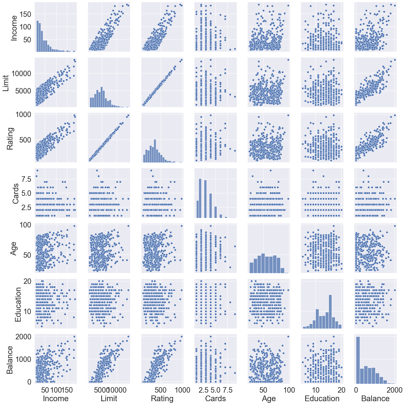
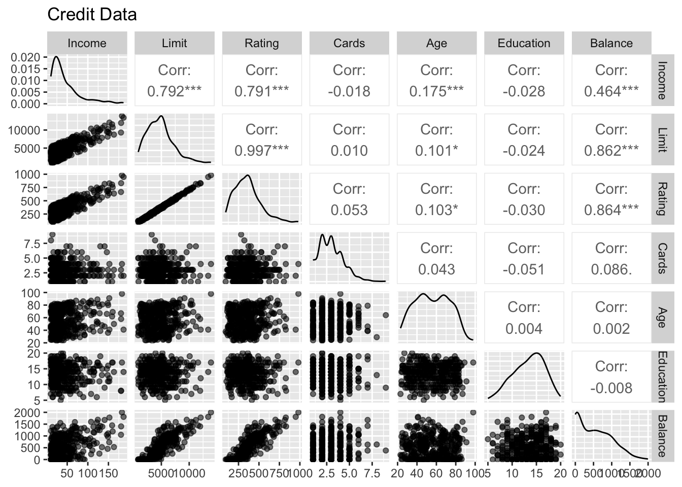
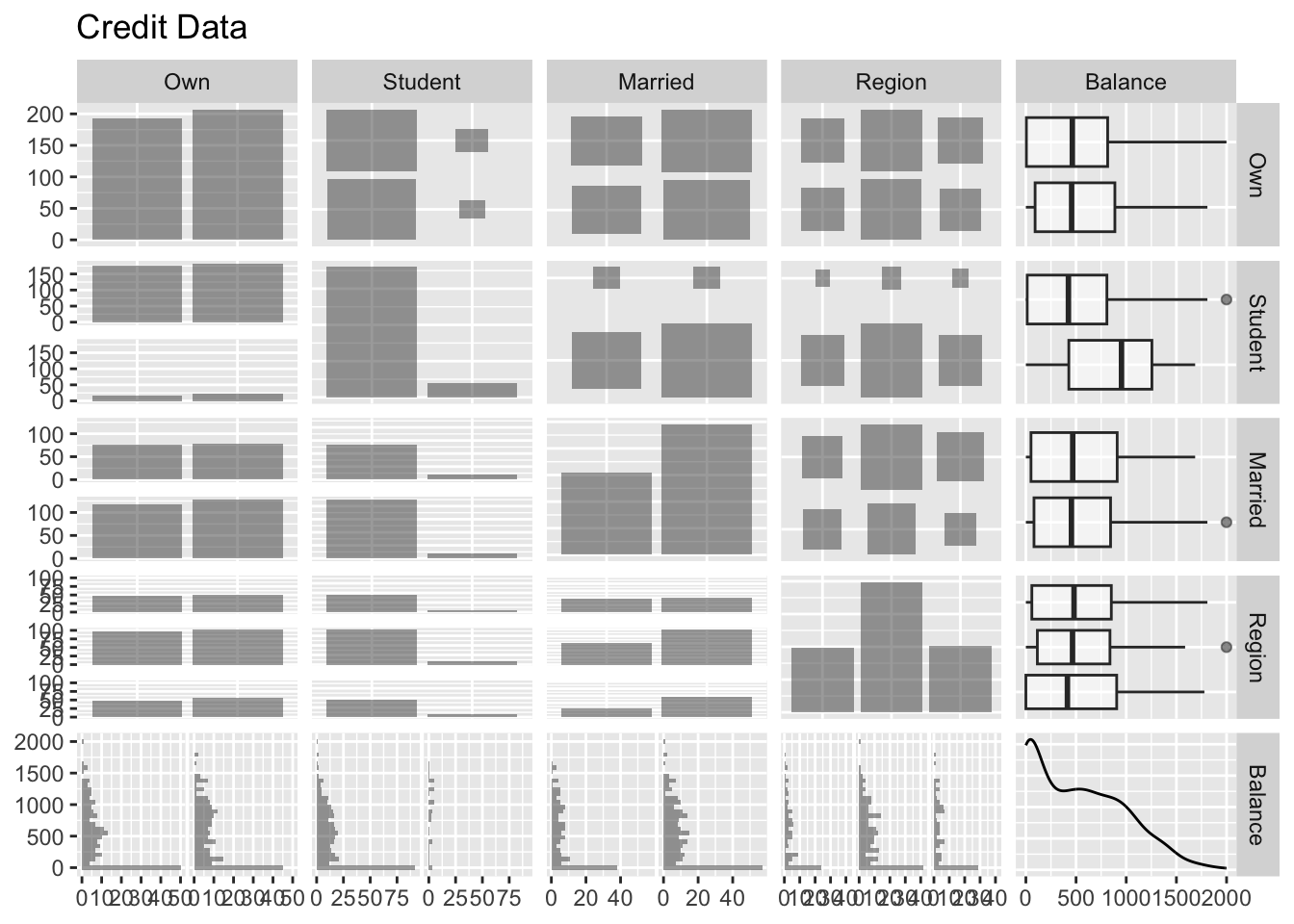
The Credit data has a mix of quantitative (Balance, Age, Cards, Education, Income, Limit, Rating) and qualitative predictors (Own, Student, Married, Region).
      Income  Limit  Rating  Cards  Age  Education  Own Student Married  \
0     14.891   3606     283      2   34         11   No      No     Yes
1    106.025   6645     483      3   82         15  Yes     Yes     Yes
2    104.593   7075     514      4   71         11   No      No      No
3    148.924   9504     681      3   36         11  Yes      No      No
4     55.882   4897     357      2   68         16   No      No     Yes
..       ...    ...     ...    ...  ...        ...  ...     ...     ...
395   12.096   4100     307      3   32         13   No      No     Yes
396   13.364   3838     296      5   65         17   No      No      No
397   57.872   4171     321      5   67         12  Yes      No     Yes
398   37.728   2525     192      1   44         13   No      No     Yes
399   18.701   5524     415      5   64          7  Yes      No      No

    Region  Balance
0    South      333
1     West      903
2     West      580
3     West      964
4    South      331
..     ...      ...
395  South      560
396   East      480
397  South      138
398  South        0
399   West      966

[400 rows x 11 columns]
# Visualization by pair plotsns.pairplot(data = Credit)
# A tibble: 400 × 11
   Income Limit Rating Cards   Age Education Own   Student Married Region
    <dbl> <dbl>  <dbl> <dbl> <dbl>     <dbl> <fct> <fct>   <fct>   <fct>
 1   14.9  3606    283     2    34        11 No    No      Yes     South
 2  106.   6645    483     3    82        15 Yes   Yes     Yes     West
 3  105.   7075    514     4    71        11 No    No      No      West
 4  149.   9504    681     3    36        11 Yes   No      No      West
 5   55.9  4897    357     2    68        16 No    No      Yes     South
 6   80.2  8047    569     4    77        10 No    No      No      South
 7   21.0  3388    259     2    37        12 Yes   No      No      East
 8   71.4  7114    512     2    87         9 No    No      No      West
 9   15.1  3300    266     5    66        13 Yes   No      No      South
10   71.1  6819    491     3    41        19 Yes   Yes     Yes     East
   Balance
     <dbl>
 1     333
 2     903
 3     580
 4     964
 5     331
 6    1151
 7     203
 8     872
 9     279
10    1350
# … with 390 more rows
By default, most software create dummy variables, also called one-hot coding, for categorical variables. Both Python (statsmodels) and R use the first level (in alphabetical order) as the base level.
# Hack to get all predictorsmy_formula ="Balance ~ "+"+".join(Credit.columns.difference(["Balance"]))# Create design matrix and response vector using R-like formulay, X = dmatrices( my_formula, data = Credit, return_type ='dataframe' )# One-hot coding for categorical variables X
# Fit linear regressionsm.OLS(y, X).fit().summary()
OLS Regression Results
Dep. Variable:
Balance
R-squared:
0.955
Model:
OLS
Adj. R-squared:
0.954
Method:
Least Squares
F-statistic:
750.3
Date:
Tue, 17 Jan 2023
Prob (F-statistic):
1.11e-253
Time:
08:51:57
Log-Likelihood:
-2398.7
No. Observations:
400
AIC:
4821.
Df Residuals:
388
BIC:
4869.
Df Model:
11
Covariance Type:
nonrobust
coef
std err
t
P>|t|
[0.025
0.975]
Intercept
-479.2079
35.774
-13.395
0.000
-549.543
-408.873
Married[T.Yes]
-8.5339
10.363
-0.824
0.411
-28.908
11.841
Own[T.Yes]
-10.6532
9.914
-1.075
0.283
-30.145
8.839
Region[T.South]
10.1070
12.210
0.828
0.408
-13.899
34.113
Region[T.West]
16.8042
14.119
1.190
0.235
-10.955
44.564
Student[T.Yes]
425.7474
16.723
25.459
0.000
392.869
458.626
Age
-0.6139
0.294
-2.088
0.037
-1.192
-0.036
Cards
17.7245
4.341
4.083
0.000
9.190
26.259
Education
-1.0989
1.598
-0.688
0.492
-4.241
2.043
Income
-7.8031
0.234
-33.314
0.000
-8.264
-7.343
Limit
0.1909
0.033
5.824
0.000
0.126
0.255
Rating
1.1365
0.491
2.315
0.021
0.171
2.102
Omnibus:
34.899
Durbin-Watson:
1.968
Prob(Omnibus):
0.000
Jarque-Bera (JB):
41.766
Skew:
0.782
Prob(JB):
8.52e-10
Kurtosis:
3.241
Cond. No.
3.87e+04
Notes: [1] Standard Errors assume that the covariance matrix of the errors is correctly specified. [2] The condition number is large, 3.87e+04. This might indicate that there are strong multicollinearity or other numerical problems.
lm(Balance ~ ., data = Credit) %>%tbl_regression() %>%bold_labels() %>%bold_p(t =0.05)
Characteristic
Beta
95% CI1
p-value
Income
-7.8
-8.3, -7.3
<0.001
Limit
0.19
0.13, 0.26
<0.001
Rating
1.1
0.17, 2.1
0.021
Cards
18
9.2, 26
<0.001
Age
-0.61
-1.2, -0.04
0.037
Education
-1.1
-4.2, 2.0
0.5
Own
No
—
—
Yes
-11
-30, 8.8
0.3
Student
No
—
—
Yes
426
393, 459
<0.001
Married
No
—
—
Yes
-8.5
-29, 12
0.4
Region
East
—
—
South
10
-14, 34
0.4
West
17
-11, 45
0.2
1 CI = Confidence Interval
There are many different ways of coding qualitative variables, measuring particular contrasts.
8 Interactions
In our previous analysis of the Advertising data, we assumed that the effect on sales of increasing one advertising medium is independent of the amount spent on the other media \[
\text{sales} \approx \beta_0 + \beta_1 \times \text{TV} + \beta_2 \times \text{radio}.
\]
But suppose that spending money on radio advertising actually increases the effectiveness of TV advertising, so that the slope term for TV should increase as radio increases.
In this situation, given a fixed budget of $100,000, spending half on radio and half on TV may increase sales more than allocating the entire amount to either TV or to radio.
In marketing, this is known as a synergy effect, and in statistics it is referred to as an interaction effect.
# Design matrix with interactiony, X_int = dmatrices('sales ~ 1 + TV * radio', data = Advertising, return_type ='dataframe' )# Fit linear regression with interactionsm.OLS(y, X_int).fit().summary()
OLS Regression Results
Dep. Variable:
sales
R-squared:
0.968
Model:
OLS
Adj. R-squared:
0.967
Method:
Least Squares
F-statistic:
1963.
Date:
Tue, 17 Jan 2023
Prob (F-statistic):
6.68e-146
Time:
08:52:03
Log-Likelihood:
-270.14
No. Observations:
200
AIC:
548.3
Df Residuals:
196
BIC:
561.5
Df Model:
3
Covariance Type:
nonrobust
coef
std err
t
P>|t|
[0.025
0.975]
Intercept
6.7502
0.248
27.233
0.000
6.261
7.239
TV
0.0191
0.002
12.699
0.000
0.016
0.022
radio
0.0289
0.009
3.241
0.001
0.011
0.046
TV:radio
0.0011
5.24e-05
20.727
0.000
0.001
0.001
Omnibus:
128.132
Durbin-Watson:
2.224
Prob(Omnibus):
0.000
Jarque-Bera (JB):
1183.719
Skew:
-2.323
Prob(JB):
9.09e-258
Kurtosis:
13.975
Cond. No.
1.80e+04
Notes: [1] Standard Errors assume that the covariance matrix of the errors is correctly specified. [2] The condition number is large, 1.8e+04. This might indicate that there are strong multicollinearity or other numerical problems.
lmod_int <-lm(sales ~1+ TV * radio, data = Advertising) summary(lmod_int)
Call:
lm(formula = sales ~ 1 + TV * radio, data = Advertising)

Residuals:
    Min      1Q  Median      3Q     Max
-6.3366 -0.4028  0.1831  0.5948  1.5246

Coefficients:
             Estimate Std. Error t value Pr(>|t|)
(Intercept) 6.750e+00  2.479e-01  27.233   <2e-16 ***
TV          1.910e-02  1.504e-03  12.699   <2e-16 ***
radio       2.886e-02  8.905e-03   3.241   0.0014 **
TV:radio    1.086e-03  5.242e-05  20.727   <2e-16 ***
---
Signif. codes:  0 '***' 0.001 '**' 0.01 '*' 0.05 '.' 0.1 ' ' 1

Residual standard error: 0.9435 on 196 degrees of freedom
Multiple R-squared:  0.9678,    Adjusted R-squared:  0.9673
F-statistic:  1963 on 3 and 196 DF,  p-value: < 2.2e-16
The results in this table suggests that the TV \(\times\) Radio interaction is important.
The \(R^2\) for the interaction model is 96.8%, compared to only 89.7% for the model that predicts sales using TV and radio without an interaction term.
This means that (96.8 - 89.7)/(100 - 89.7) = 69% of the variability in sales that remains after fitting the additive model has been explained by the interaction term.
The coefficient estimates in the table suggest that an increase in TV advertising of $1,000 is associated with increased sales of \[
(\hat \beta_1 + \hat \beta_3 \times \text{radio}) \times 1000 = 19 + 1.1 \times \text{radio units}.
\]
An increase in radio advertising of $1,000 will be associated with an increase in sales of \[
(\hat \beta_2 + \hat \beta_3 \times \text{TV}) \times 1000 = 29 + 1.1 \times \text{TV units}.
\]
Sometimes it is the case that an interaction term has a very small p-value, but the associated main effects (in this case, TV and radio) do not.
The hierarchy principle staties
If we include an interaction in a model, we should also include the main effects, even if the \(p\)-values associated with their coefficients are not significant.
The rationale for this principle is that interactions are hard to interpret in a model without main effects – their meaning is changed. Specifically, the interaction terms still contain main effects, if the model has no main effect terms.
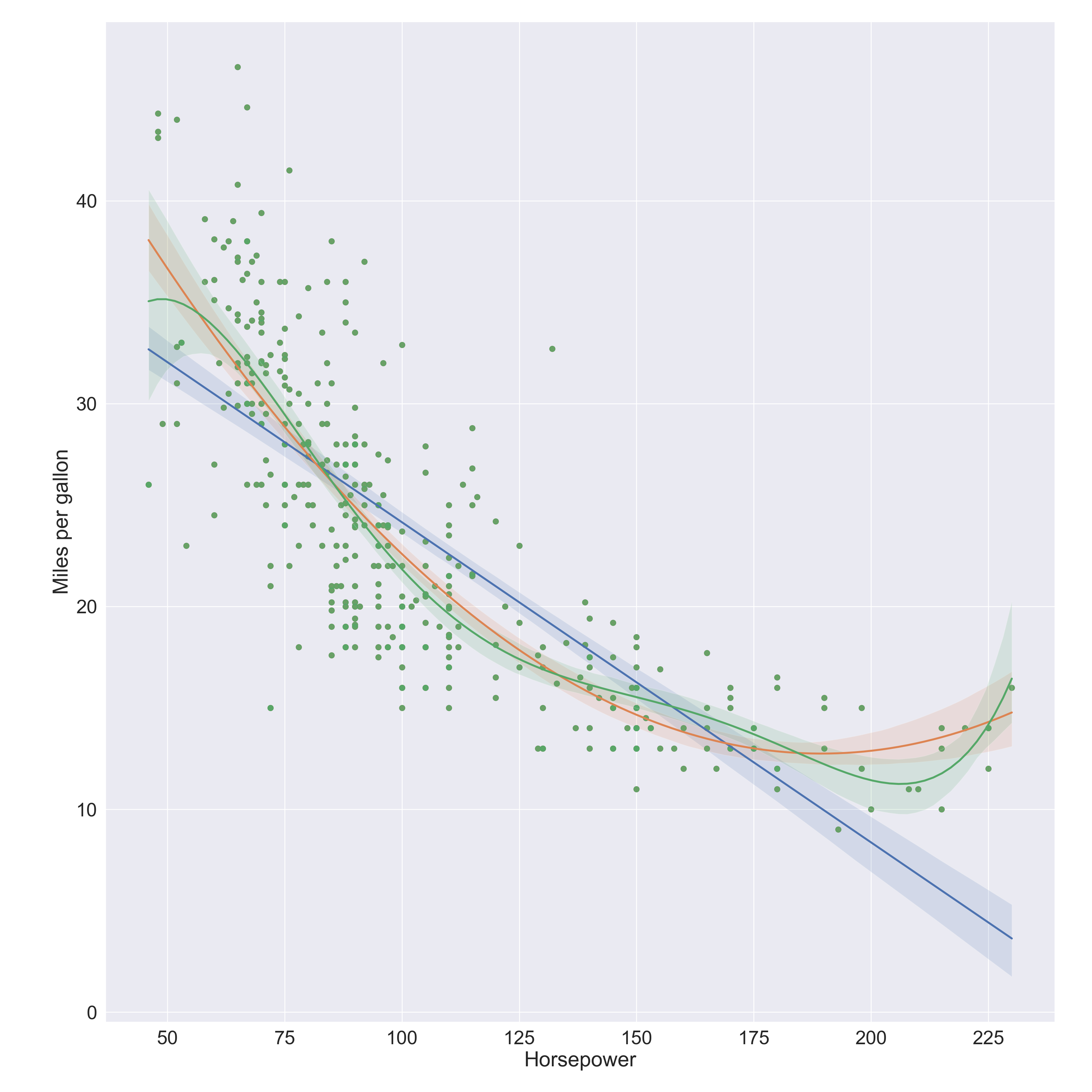
plt.clf()# Linear fitax = sns.regplot( data = Auto, x ='horsepower', y ='mpg', order =1 )# Quadratic fit sns.regplot( data = Auto, x ='horsepower', y ='mpg', order =2, ax = ax )# 5-degree fit sns.regplot( data = Auto, x ='horsepower', y ='mpg', order =5, ax = ax )ax.set( xlabel ='Horsepower', ylabel ='Miles per gallon')
# Linear fitlm(mpg ~ horsepower, data = Auto) %>%summary()
Call:
lm(formula = mpg ~ horsepower, data = Auto)

Residuals:
     Min       1Q   Median       3Q      Max
-13.5710  -3.2592  -0.3435   2.7630  16.9240

Coefficients:
             Estimate Std. Error t value Pr(>|t|)
(Intercept) 39.935861   0.717499   55.66   <2e-16 ***
horsepower  -0.157845   0.006446  -24.49   <2e-16 ***
---
Signif. codes:  0 '***' 0.001 '**' 0.01 '*' 0.05 '.' 0.1 ' ' 1

Residual standard error: 4.906 on 390 degrees of freedom
Multiple R-squared:  0.6059,    Adjusted R-squared:  0.6049
F-statistic: 599.7 on 1 and 390 DF,  p-value: < 2.2e-16
# Degree 2lm(mpg ~poly(horsepower, 2), data = Auto) %>%summary()
Call:
lm(formula = mpg ~ poly(horsepower, 2), data = Auto)

Residuals:
     Min       1Q   Median       3Q      Max
-14.7135  -2.5943  -0.0859   2.2868  15.8961

Coefficients:
                      Estimate Std. Error t value Pr(>|t|)
(Intercept)            23.4459     0.2209  106.13   <2e-16 ***
poly(horsepower, 2)1 -120.1377     4.3739  -27.47   <2e-16 ***
poly(horsepower, 2)2   44.0895     4.3739   10.08   <2e-16 ***
---
Signif. codes:  0 '***' 0.001 '**' 0.01 '*' 0.05 '.' 0.1 ' ' 1

Residual standard error: 4.374 on 389 degrees of freedom
Multiple R-squared:  0.6876,    Adjusted R-squared:  0.686
F-statistic:   428 on 2 and 389 DF,  p-value: < 2.2e-16
# Degree 5lm(mpg ~poly(horsepower, 5), data = Auto) %>%summary()
Call:
lm(formula = mpg ~ poly(horsepower, 5), data = Auto)

Residuals:
     Min       1Q   Median       3Q      Max
-15.4326  -2.5285  -0.2925   2.1750  15.9730

Coefficients:
                      Estimate Std. Error t value Pr(>|t|)
(Intercept)            23.4459     0.2185 107.308  < 2e-16 ***
poly(horsepower, 5)1 -120.1377     4.3259 -27.772  < 2e-16 ***
poly(horsepower, 5)2   44.0895     4.3259  10.192  < 2e-16 ***
poly(horsepower, 5)3   -3.9488     4.3259  -0.913  0.36190
poly(horsepower, 5)4   -5.1878     4.3259  -1.199  0.23117
poly(horsepower, 5)5   13.2722     4.3259   3.068  0.00231 **
---
Signif. codes:  0 '***' 0.001 '**' 0.01 '*' 0.05 '.' 0.1 ' ' 1

Residual standard error: 4.326 on 386 degrees of freedom
Multiple R-squared:  0.6967,    Adjusted R-squared:  0.6928
F-statistic: 177.4 on 5 and 386 DF,  p-value: < 2.2e-16
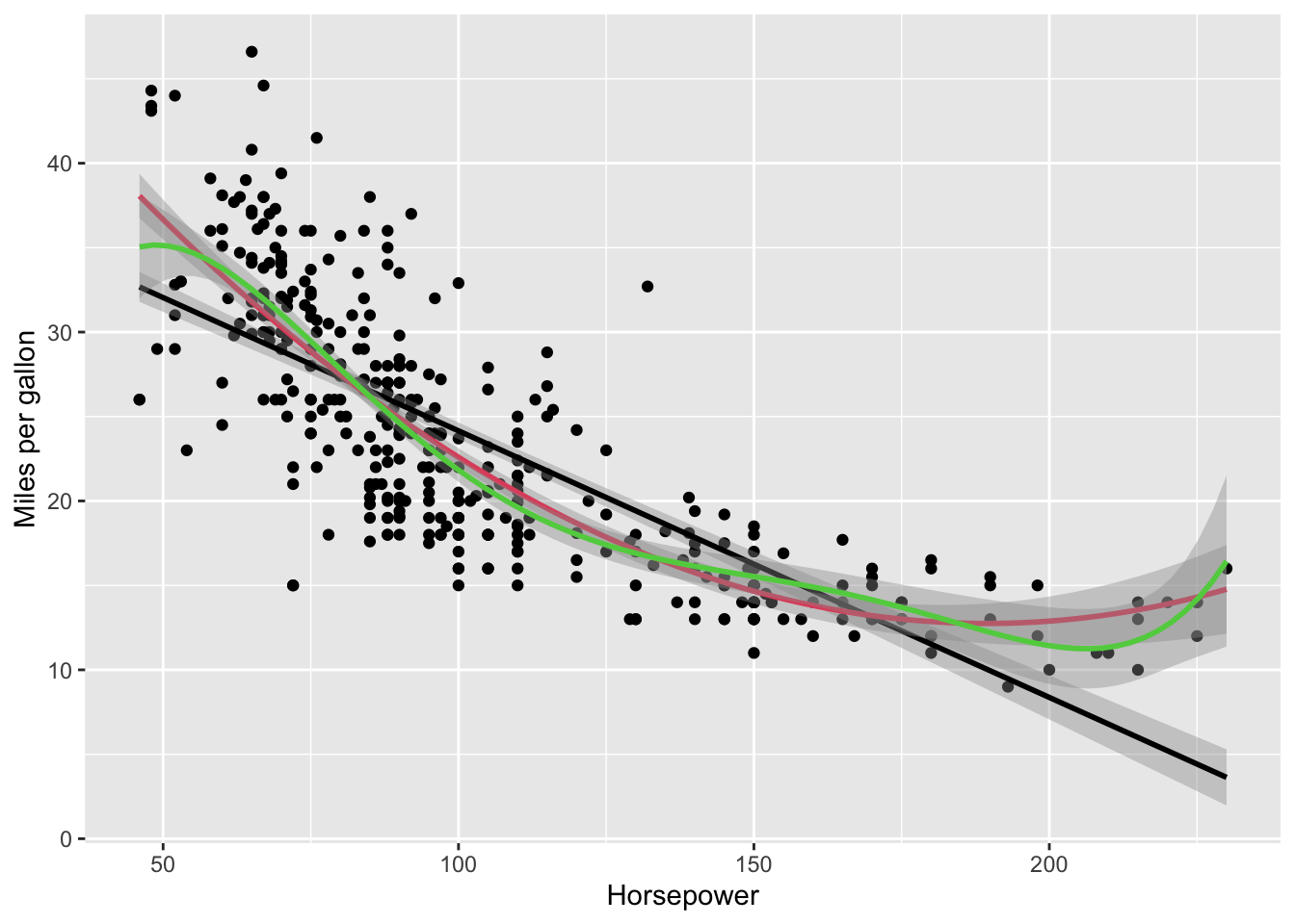
ggplot(data = Auto, mapping =aes(x = horsepower, y = mpg)) +geom_point() +geom_smooth(method = lm, color =1) +geom_smooth(method = lm, formula = y ~poly(x, 2), color =2) +geom_smooth(method = lm, formula = y ~poly(x, 5), color =3) +labs(x ="Horsepower", y ="Miles per gallon")
10 What we did not cover
Outliers.
Non-constant variance of error terms.
High leverage points.
Collinearity.
See ISL Section 3.3.3.
11 Generalizations of linear models
In much of the rest of this course, we discuss methods that expand the scope of linear models and how they are fit.
Classification problems: logistic regression, discriminant analysis, support vector machines.