Machine Learning Workflow: Classifiers With Nonlinear Features

Econ 425T

Display system information for reproducibility.

Python

import IPython
print(IPython.sys_info())

{'commit_hash': 'add5877a4',
 'commit_source': 'installation',
 'default_encoding': 'utf-8',
 'ipython_path': '/Library/Frameworks/Python.framework/Versions/3.10/lib/python3.10/site-packages/IPython',
 'ipython_version': '8.8.0',
 'os_name': 'posix',
 'platform': 'macOS-10.16-x86_64-i386-64bit',
 'sys_executable': '/Library/Frameworks/Python.framework/Versions/3.10/bin/python3',
 'sys_platform': 'darwin',
 'sys_version': '3.10.9 (v3.10.9:1dd9be6584, Dec  6 2022, 14:37:36) [Clang '
                '13.0.0 (clang-1300.0.29.30)]'}

R

sessionInfo()

R version 4.2.2 (2022-10-31)
Platform: x86_64-apple-darwin17.0 (64-bit)
Running under: macOS Big Sur ... 10.16

Matrix products: default
BLAS:   /Library/Frameworks/R.framework/Versions/4.2/Resources/lib/libRblas.0.dylib
LAPACK: /Library/Frameworks/R.framework/Versions/4.2/Resources/lib/libRlapack.dylib

locale:
[1] en_US.UTF-8/en_US.UTF-8/en_US.UTF-8/C/en_US.UTF-8/en_US.UTF-8

attached base packages:
[1] stats     graphics  grDevices utils     datasets  methods   base     

loaded via a namespace (and not attached):
 [1] Rcpp_1.0.9        here_1.0.1        lattice_0.20-45   png_0.1-8        
 [5] rprojroot_2.0.3   digest_0.6.30     grid_4.2.2        lifecycle_1.0.3  
 [9] jsonlite_1.8.4    magrittr_2.0.3    evaluate_0.18     rlang_1.0.6      
[13] stringi_1.7.8     cli_3.4.1         rstudioapi_0.14   Matrix_1.5-1     
[17] reticulate_1.26   vctrs_0.5.1       rmarkdown_2.18    tools_4.2.2      
[21] stringr_1.5.0     glue_1.6.2        htmlwidgets_1.6.0 xfun_0.35        
[25] yaml_2.3.6        fastmap_1.1.0     compiler_4.2.2    htmltools_0.5.4  
[29] knitr_1.41       

1 Overview

We illustrate the typical machine learning workflow for regression problems using the Default data set from R ISLR2 package. Our goal is to classify whether a credit card customer will default or not. The steps are

1. Initial splitting to test and non-test sets.

2. Pre-processing of data: one-hot-encoder for categorical variables, add nonlinear features (B-splines) for some continuous predictors.

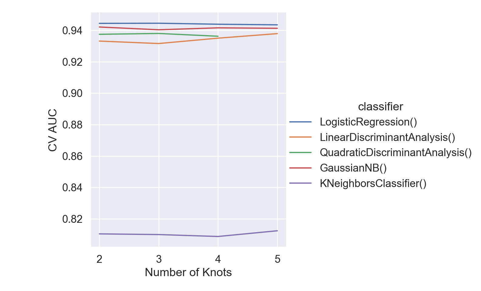
3. Choose a set of candidate classifiers: logistic regression, LDA, QDA, NB, KNN.

4. Tune the hyper-parameter(s) (n_knots in SplineTransformer, classifier) using 10-fold cross-validation (CV) on the non-test data.

5. Choose the best model by CV and refit it on the whole non-test data.

6. Final classification on the test data.

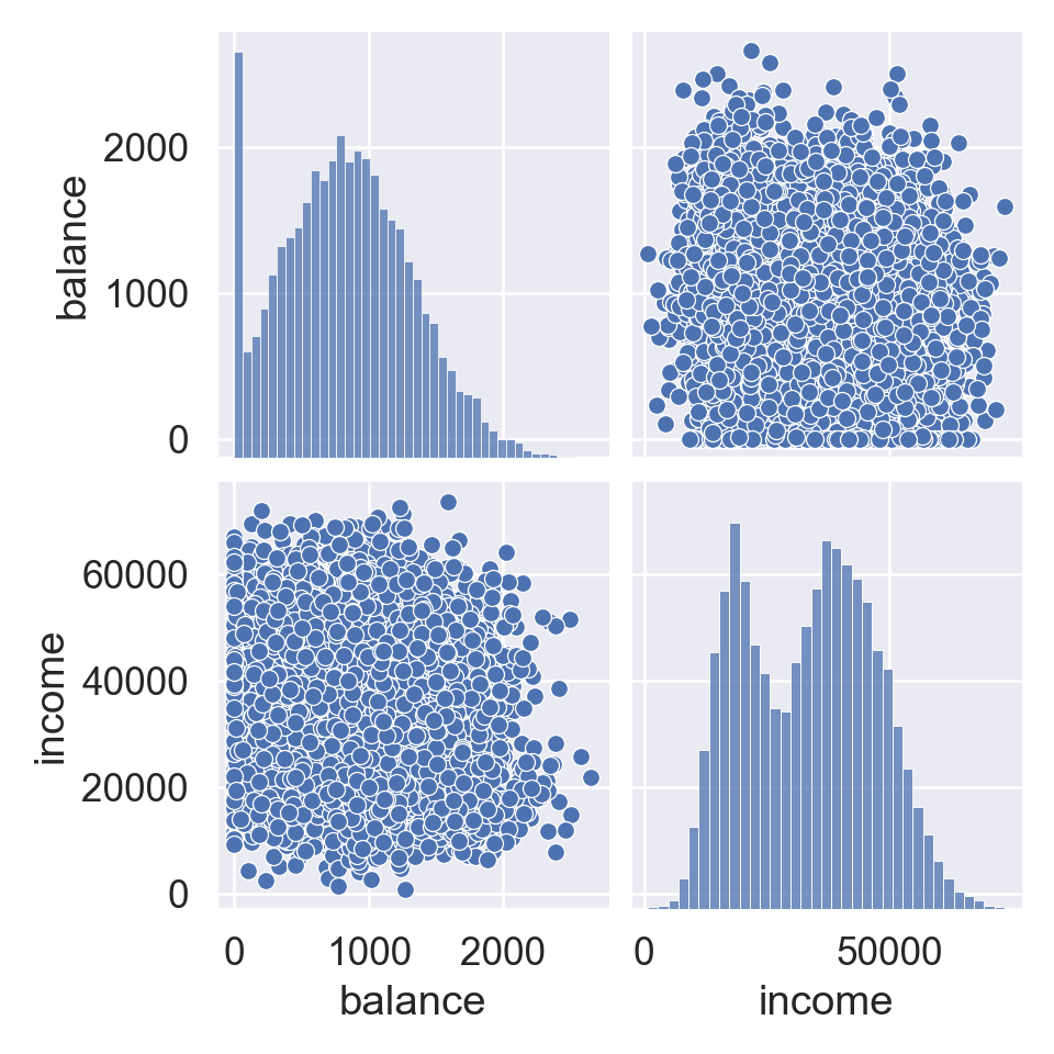
2 Default data

A documentation of the Default data is here. The goal is to classify whether a credit card customer will default or not.

Python

# Load the pandas library
import pandas as pd
# Load numpy for array manipulation
import numpy as np
# Load seaborn plotting library
import seaborn as sns
import matplotlib.pyplot as plt

# Set font sizes in plots
sns.set(font_scale = 1.2)
# Display all columns
pd.set_option('display.max_columns', None)

Default = pd.read_csv("../data/Default.csv")
Default

     default student      balance        income
0         No      No   729.526495  44361.625074
1         No     Yes   817.180407  12106.134700
2         No      No  1073.549164  31767.138947
3         No      No   529.250605  35704.493935
4         No      No   785.655883  38463.495879
...      ...     ...          ...           ...
9995      No      No   711.555020  52992.378914
9996      No      No   757.962918  19660.721768
9997      No      No   845.411989  58636.156984
9998      No      No  1569.009053  36669.112365
9999      No     Yes   200.922183  16862.952321

[10000 rows x 4 columns]

# Numerical summaries
Default.describe()

            balance        income
count  10000.000000  10000.000000
mean     835.374886  33516.981876
std      483.714985  13336.639563
min        0.000000    771.967729
25%      481.731105  21340.462903
50%      823.636973  34552.644802
75%     1166.308386  43807.729272
max     2654.322576  73554.233495

Graphical summary:

# Graphical summaries
plt.figure()
sns.pairplot(data = Default);
plt.show()

R

library(GGally)
library(ISLR2)
library(tidymodels)
library(tidyverse)

Default <- as_tibble(Default) %>%
  print(width = Inf)

# A tibble: 10,000 × 4
   default student balance income
   <fct>   <fct>     <dbl>  <dbl>
 1 No      No         730. 44362.
 2 No      Yes        817. 12106.
 3 No      No        1074. 31767.
 4 No      No         529. 35704.
 5 No      No         786. 38463.
 6 No      Yes        920.  7492.
 7 No      No         826. 24905.
 8 No      Yes        809. 17600.
 9 No      No        1161. 37469.
10 No      No           0  29275.
# … with 9,990 more rows

# Numerical summaries
summary(Default)

 default    student       balance           income     
 No :9667   No :7056   Min.   :   0.0   Min.   :  772  
 Yes: 333   Yes:2944   1st Qu.: 481.7   1st Qu.:21340  
                       Median : 823.6   Median :34553  
                       Mean   : 835.4   Mean   :33517  
                       3rd Qu.:1166.3   3rd Qu.:43808  
                       Max.   :2654.3   Max.   :73554  

Graphical summary.

# Graphical summaries
ggpairs(
  data = Default, 
  mapping = aes(alpha = 0.25), 
  lower = list(continuous = "smooth")
  ) + 
  labs(title = "Default Data")

3 Initial split into test and non-test sets

It is a good idea to keep the proportions of default = 'Yes' to be roughly same between test and non-test data.

Python

from sklearn.model_selection import train_test_split

Default_other, Default_test = train_test_split(
  Default, 
  train_size = 0.75,
  random_state = 425, # seed
  stratify = Default.default
  )
Default_test.shape

(2500, 4)

Default_other.shape

(7500, 4)

Separate \(X\) and \(y\).

# Non-test X and y
X_other = Default_other[['balance', 'income', 'student']]
y_other = Default_other.default
# Test X and y
X_test = Default_test[['balance', 'income', 'student']]
y_test = Default_test.default

R

# For reproducibility
set.seed(425)
data_split <- initial_split(
  Wage, 
  # # stratify by percentiles
  # strata = "Salary", 
  prop = 0.75
  )

Wage_other <- training(data_split)
dim(Wage_other)
Wage_test <- testing(data_split)
dim(Wage_test)

4 Preprocessing (Python) or recipe (R)

Python

Pre-processor for one-hot coding of categorical variables and then standardizing all numeric predictors.

from sklearn.preprocessing import OneHotEncoder, StandardScaler, SplineTransformer
from sklearn.compose import ColumnTransformer
from sklearn.pipeline import Pipeline

# Transformer for numeric variables
numeric_tf = Pipeline(steps = [
  # ("scalar", StandardScaler()),
  ("bspline", SplineTransformer(degree = 3, extrapolation = 'linear'))
])
# Transformer for categorical variables
categorical_tf = Pipeline(steps = [
  ("encoder", OneHotEncoder(drop = 'first'))
])

# Column transformer
col_tf = ColumnTransformer(transformers = [
  ('num', numeric_tf, ['balance', 'income']),
  ('cat', categorical_tf, ['student'])
])

R

norm_recipe <- 
  recipe(
    wage ~ year + age + education, 
    data = Wage_other
  ) %>%
  # create traditional dummy variables
  step_dummy(all_nominal()) %>%
  # zero-variance filter
  step_zv(all_predictors()) %>% 
  # B-splines of age
  step_bs(age, deg_free = 5) %>%
  # B-splines of year
  step_bs(year, deg_free = 4) %>%
  # center and scale numeric data
  step_normalize(all_predictors()) %>%
  # estimate the means and standard deviations
  prep(training = Wage_other, retain = TRUE)
norm_recipe

5 Model

Let’s skip this step for now, because the model (or classifer) itself is being tuned by CV.

Python

R

enet_mod <- 
  # mixture = 0 (ridge), mixture = 1 (lasso)
  linear_reg(penalty = tune(), mixture = tune()) %>% 
  set_engine("glmnet")
enet_mod

6 Pipeline (Python) or workflow (R)

Here we bundle the preprocessing step (Python) or recipe (R) and model. Again remember KNN is a placeholder here. Later we will choose the better classifier according to cross validation.

Python

from sklearn.neighbors import KNeighborsClassifier

pipe = Pipeline(steps = [
  ("col_tf", col_tf),
  ("model", KNeighborsClassifier())
  ])
pipe

Pipeline(steps=[('col_tf',
                 ColumnTransformer(transformers=[('num',
                                                  Pipeline(steps=[('bspline',
                                                                   SplineTransformer(extrapolation='linear'))]),
                                                  ['balance', 'income']),
                                                 ('cat',
                                                  Pipeline(steps=[('encoder',
                                                                   OneHotEncoder(drop='first'))]),
                                                  ['student'])])),
                ('model', KNeighborsClassifier())])

In a Jupyter environment, please rerun this cell to show the HTML representation or trust the notebook.
On GitHub, the HTML representation is unable to render, please try loading this page with nbviewer.org.

R

lr_wf <- 
  workflow() %>%
  add_model(enet_mod) %>%
  add_recipe(norm_recipe)
lr_wf

7 Tuning grid

Set up the 2D grid for tuning.

Python

from sklearn.linear_model import LogisticRegression
from sklearn.discriminant_analysis import LinearDiscriminantAnalysis, QuadraticDiscriminantAnalysis
from sklearn.naive_bayes import GaussianNB

# Tune hyper-parameter(s)
nknots_grid = np.array(range(2, 6))
classifers = [
  LogisticRegression(),
  LinearDiscriminantAnalysis(),
  QuadraticDiscriminantAnalysis(),
  GaussianNB(),
  KNeighborsClassifier(n_neighbors = 5)
  ]
tuned_parameters = {
  "col_tf__num__bspline__n_knots": nknots_grid,
  "model": classifers
  }
tuned_parameters  

{'col_tf__num__bspline__n_knots': array([2, 3, 4, 5]), 'model': [LogisticRegression(), LinearDiscriminantAnalysis(), QuadraticDiscriminantAnalysis(), GaussianNB(), KNeighborsClassifier()]}

R

param_grid <-grid_regular(
  penalty(range = c(-5, 0), trans = log10_trans()), 
  mixture(range = c(0, 1)),
  levels = c(penalty = 50, mixture = 6)
  )
param_grid

8 Cross-validation (CV)

Python

Set up CV partitions and CV criterion. Again it’s a good idea to keep the case proportions roughly same between splits. According to the GridSearchCV documentation, StratifiedKFold is used automatically.

from sklearn.model_selection import GridSearchCV

# Set up CV
n_folds = 10
search = GridSearchCV(
  pipe,
  tuned_parameters,
  cv = n_folds, 
  scoring = "roc_auc",
  # Refit the best model on the whole data set
  refit = True
  )

Fit CV. This is typically the most time-consuming step.

# Fit CV
search.fit(X_other, y_other)

GridSearchCV(cv=10,
             estimator=Pipeline(steps=[('col_tf',
                                        ColumnTransformer(transformers=[('num',
                                                                         Pipeline(steps=[('bspline',
                                                                                          SplineTransformer(extrapolation='linear'))]),
                                                                         ['balance',
                                                                          'income']),
                                                                        ('cat',
                                                                         Pipeline(steps=[('encoder',
                                                                                          OneHotEncoder(drop='first'))]),
                                                                         ['student'])])),
                                       ('model', KNeighborsClassifier())]),
             param_grid={'col_tf__num__bspline__n_knots': array([2, 3, 4, 5]),
                         'model': [LogisticRegression(),
                                   LinearDiscriminantAnalysis(),
                                   QuadraticDiscriminantAnalysis(),
                                   GaussianNB(), KNeighborsClassifier()]},
             scoring='roc_auc')

In a Jupyter environment, please rerun this cell to show the HTML representation or trust the notebook.
On GitHub, the HTML representation is unable to render, please try loading this page with nbviewer.org.

Visualize CV results.

Code

cv_res = pd.DataFrame({
  "nknots": np.array(search.cv_results_["param_col_tf__num__bspline__n_knots"]),
  "classifier": np.array(search.cv_results_["param_model"]),
  "aucroc": search.cv_results_["mean_test_score"]
  })

plt.figure()
sns.relplot(
  kind = "line",
  data = cv_res,
  x = "nknots",
  y = "aucroc",
  hue = "classifier"
  ).set(
    xlabel = "Number of Knots",
    ylabel = "CV AUC"
);
plt.show()

Best CV AUC-ROC:

search.best_score_

0.9444910344827585

R

Set cross-validation partitions.

set.seed(250)
folds <- vfold_cv(Wage_other, v = 10)
folds

Fit cross-validation.

enet_fit <- 
  lr_wf %>%
  tune_grid(
    resamples = folds,
    grid = param_grid,
    )
enet_fit

Visualize CV criterion.

enet_fit %>%
  collect_metrics() %>%
  print(width = Inf) %>%
  filter(.metric == "rmse") %>%
  ggplot(mapping = aes(x = penalty, y = mean)) + 
  geom_point() + 
  geom_line(aes(group = mixture)) + 
  labs(x = "Penalty", y = "CV RMSE") + 
  scale_x_log10(labels = scales::label_number())

Show the top 5 models (\(\lambda\) values)

enet_fit %>%
  show_best("rmse")

Let’s select the best model

best_enet <- enet_fit %>%
  select_best("rmse")
best_enet

9 Finalize our model

Now we are done tuning. Finally, let’s fit this final model to the whole training data and use our test data to estimate the model performance we expect to see with new data.

Python

Since we called GridSearchCV with refit = True, the best model fit on the whole non-test data is readily available.

search.best_estimator_

Pipeline(steps=[('col_tf',
                 ColumnTransformer(transformers=[('num',
                                                  Pipeline(steps=[('bspline',
                                                                   SplineTransformer(extrapolation='linear',
                                                                                     n_knots=3))]),
                                                  ['balance', 'income']),
                                                 ('cat',
                                                  Pipeline(steps=[('encoder',
                                                                   OneHotEncoder(drop='first'))]),
                                                  ['student'])])),
                ('model', LogisticRegression())])

In a Jupyter environment, please rerun this cell to show the HTML representation or trust the notebook.
On GitHub, the HTML representation is unable to render, please try loading this page with nbviewer.org.

The final AUC on the test set is

from sklearn.metrics import roc_auc_score

roc_auc_score(
  y_test, 
  search.best_estimator_.predict_proba(X_test)[:, 1]
  )

0.9648772998489614

R

# Final workflow
final_wf <- lr_wf %>%
  finalize_workflow(best_enet)
final_wf

# Fit the whole training set, then predict the test cases
final_fit <- 
  final_wf %>%
  last_fit(data_split)
final_fit

# Test metrics
final_fit %>% collect_metrics()