R version 4.2.2 (2022-10-31)
Platform: x86_64-apple-darwin17.0 (64-bit)
Running under: macOS Big Sur ... 10.16

Matrix products: default
BLAS:   /Library/Frameworks/R.framework/Versions/4.2/Resources/lib/libRblas.0.dylib
LAPACK: /Library/Frameworks/R.framework/Versions/4.2/Resources/lib/libRlapack.dylib

locale:
[1] en_US.UTF-8/en_US.UTF-8/en_US.UTF-8/C/en_US.UTF-8/en_US.UTF-8

attached base packages:
[1] stats     graphics  grDevices utils     datasets  methods   base

loaded via a namespace (and not attached):
 [1] Rcpp_1.0.9        here_1.0.1        lattice_0.20-45   png_0.1-8
 [5] rprojroot_2.0.3   digest_0.6.30     grid_4.2.2        lifecycle_1.0.3
 [9] jsonlite_1.8.4    magrittr_2.0.3    evaluate_0.18     rlang_1.0.6
[13] stringi_1.7.8     cli_3.4.1         rstudioapi_0.14   Matrix_1.5-1
[17] reticulate_1.26   vctrs_0.5.1       rmarkdown_2.18    tools_4.2.2
[21] stringr_1.5.0     glue_1.6.2        htmlwidgets_1.6.0 xfun_0.35
[25] yaml_2.3.6        fastmap_1.1.0     compiler_4.2.2    htmltools_0.5.4
[29] knitr_1.41
1 Overview
In linear regression (ISL 3), we assume \[
Y = \beta_0 + \beta_1 X_1 + \cdots + \beta_p X_p + \epsilon.
\]
In this lecture, we discuss some ways in which the simple linear model can be improved, by replacing ordinary least squares fitting with some alternative fitting procedures.
Why consider alternatives to least squares?
Prediction accuracy: especially when \(p > n\), to control the variance.
Model interpretability: By removing irrelevant features - that is, by setting the corresponding coefficient estimates to zero - we can obtain a model that is more easily interpreted. We will present some approaches for automatically performing feature selection.
Three classes of methods:
Subset selection: We identify a subset of the \(p\) predictors that we believe to be related to the response. We then fit a model using least squares on the reduced set of variables.
Shrinkage: We fit a model involving all \(p\) predictors, but the estimated coefficients are shrunken towards zero relative to the least squares estimates. This shrinkage (also known as regularization) has the effect of reducing variance and can also perform variable selection.
Dimension reduction: We project the \(p\) predictors into an \(M\)-dimensional subspace, where \(M < p\). This is achieved by computing \(M\) different linear combinations, or projections, of the variables. Then these \(M\) projections are used as predictors to fit a linear regression model by least squares.
2Credit data set
We will use the Credit data set as a running example. A documentation of this data set is at here.
# Load the pandas libraryimport pandas as pd# Load numpy for array manipulationimport numpy as np# Load seaborn plotting libraryimport seaborn as snsimport matplotlib.pyplot as plt# Set font sizes in plotssns.set(font_scale =2)# Display all columnspd.set_option('display.max_columns', None)# Import Advertising dataCredit = pd.read_csv("../data/Credit.csv")Credit
      Income  Limit  Rating  Cards  Age  Education  Own Student Married  \
0     14.891   3606     283      2   34         11   No      No     Yes
1    106.025   6645     483      3   82         15  Yes     Yes     Yes
2    104.593   7075     514      4   71         11   No      No      No
3    148.924   9504     681      3   36         11  Yes      No      No
4     55.882   4897     357      2   68         16   No      No     Yes
..       ...    ...     ...    ...  ...        ...  ...     ...     ...
395   12.096   4100     307      3   32         13   No      No     Yes
396   13.364   3838     296      5   65         17   No      No      No
397   57.872   4171     321      5   67         12  Yes      No     Yes
398   37.728   2525     192      1   44         13   No      No     Yes
399   18.701   5524     415      5   64          7  Yes      No      No

    Region  Balance
0    South      333
1     West      903
2     West      580
3     West      964
4    South      331
..     ...      ...
395  South      560
396   East      480
397  South      138
398  South        0
399   West      966

[400 rows x 11 columns]
# Numerical summaryCredit.describe()
           Income         Limit      Rating       Cards         Age  \
count  400.000000    400.000000  400.000000  400.000000  400.000000
mean    45.218885   4735.600000  354.940000    2.957500   55.667500
std     35.244273   2308.198848  154.724143    1.371275   17.249807
min     10.354000    855.000000   93.000000    1.000000   23.000000
25%     21.007250   3088.000000  247.250000    2.000000   41.750000
50%     33.115500   4622.500000  344.000000    3.000000   56.000000
75%     57.470750   5872.750000  437.250000    4.000000   70.000000
max    186.634000  13913.000000  982.000000    9.000000   98.000000

        Education      Balance
count  400.000000   400.000000
mean    13.450000   520.015000
std      3.125207   459.758877
min      5.000000     0.000000
25%     11.000000    68.750000
50%     14.000000   459.500000
75%     16.000000   863.000000
max     20.000000  1999.000000
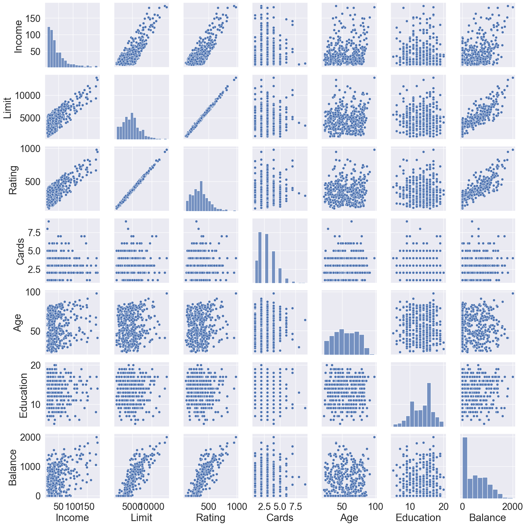
# Graphical summarysns.pairplot(data = Credit)
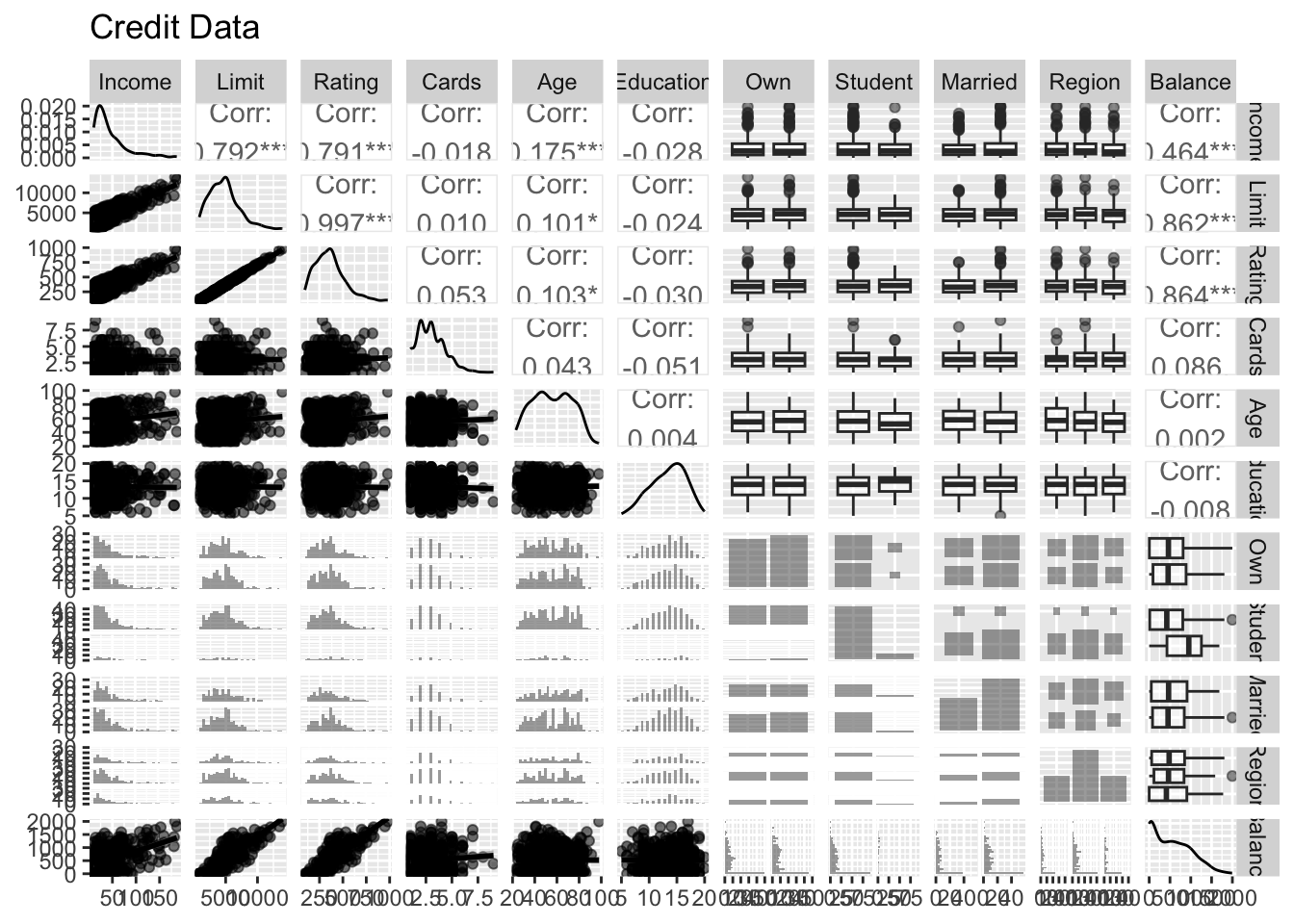
library(GGally) # ggpairs functionlibrary(ISLR2)library(tidyverse)# Cast to tibbleCredit <-as_tibble(Credit) %>%print(width =Inf)
# A tibble: 400 × 11
   Income Limit Rating Cards   Age Education Own   Student Married Region
    <dbl> <dbl>  <dbl> <dbl> <dbl>     <dbl> <fct> <fct>   <fct>   <fct>
 1   14.9  3606    283     2    34        11 No    No      Yes     South
 2  106.   6645    483     3    82        15 Yes   Yes     Yes     West
 3  105.   7075    514     4    71        11 No    No      No      West
 4  149.   9504    681     3    36        11 Yes   No      No      West
 5   55.9  4897    357     2    68        16 No    No      Yes     South
 6   80.2  8047    569     4    77        10 No    No      No      South
 7   21.0  3388    259     2    37        12 Yes   No      No      East
 8   71.4  7114    512     2    87         9 No    No      No      West
 9   15.1  3300    266     5    66        13 Yes   No      No      South
10   71.1  6819    491     3    41        19 Yes   Yes     Yes     East
   Balance
     <dbl>
 1     333
 2     903
 3     580
 4     964
 5     331
 6    1151
 7     203
 8     872
 9     279
10    1350
# … with 390 more rows
# Numerical summarysummary(Credit)
     Income           Limit           Rating          Cards
 Min.   : 10.35   Min.   :  855   Min.   : 93.0   Min.   :1.000
 1st Qu.: 21.01   1st Qu.: 3088   1st Qu.:247.2   1st Qu.:2.000
 Median : 33.12   Median : 4622   Median :344.0   Median :3.000
 Mean   : 45.22   Mean   : 4736   Mean   :354.9   Mean   :2.958
 3rd Qu.: 57.47   3rd Qu.: 5873   3rd Qu.:437.2   3rd Qu.:4.000
 Max.   :186.63   Max.   :13913   Max.   :982.0   Max.   :9.000
      Age          Education      Own      Student   Married     Region
 Min.   :23.00   Min.   : 5.00   No :193   No :360   No :155   East : 99
 1st Qu.:41.75   1st Qu.:11.00   Yes:207   Yes: 40   Yes:245   South:199
 Median :56.00   Median :14.00                                 West :102
 Mean   :55.67   Mean   :13.45
 3rd Qu.:70.00   3rd Qu.:16.00
 Max.   :98.00   Max.   :20.00
    Balance
 Min.   :   0.00
 1st Qu.:  68.75
 Median : 459.50
 Mean   : 520.01
 3rd Qu.: 863.00
 Max.   :1999.00
Let \(\mathcal{M}_0\) be the null model, which contains no predictors besides the intercept. This model simply predicts the sample mean for each observation.
For \(k = 1,2, \ldots, p\):
Fit all \(\binom{p}{k}\) models that contain exactly \(k\) predictors.
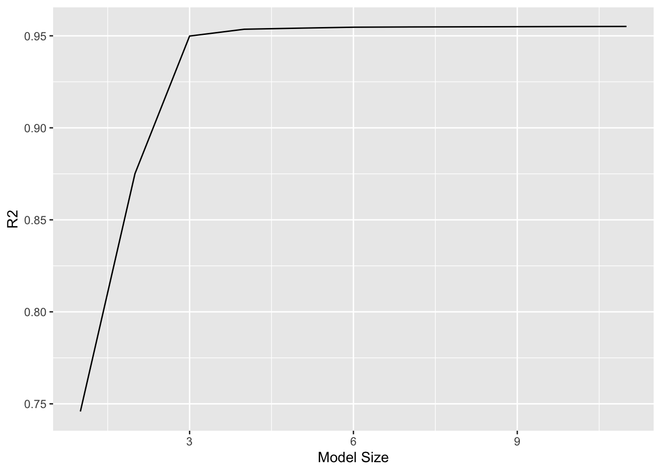
Pick the best among these \(\binom{p}{k}\) models, and call it \(\mathcal{M}_k\). Here best is defined as having the smallest RSS, or equivalently largest \(R^2\).
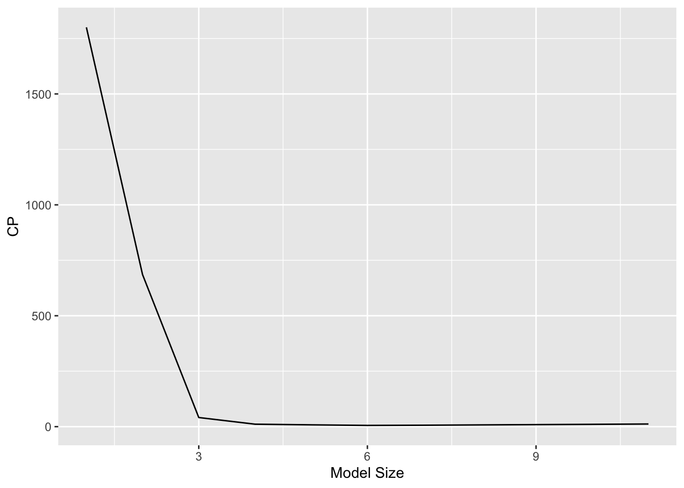
Select a single best model from among \(\mathcal{M}_0, \mathcal{M}_1, \ldots, \mathcal{M}_p\) using cross-validated prediction error, \(C_p\) (AIC), BIC, or adjusted \(R^2\).
Adjusted \(R^2\) chooses the best model of size 7: income, limit, rating, cards, age, student and own.
\(C_p\) (and AIC) chooses the best model of size 6: income, limit, rating, cards, age and student.
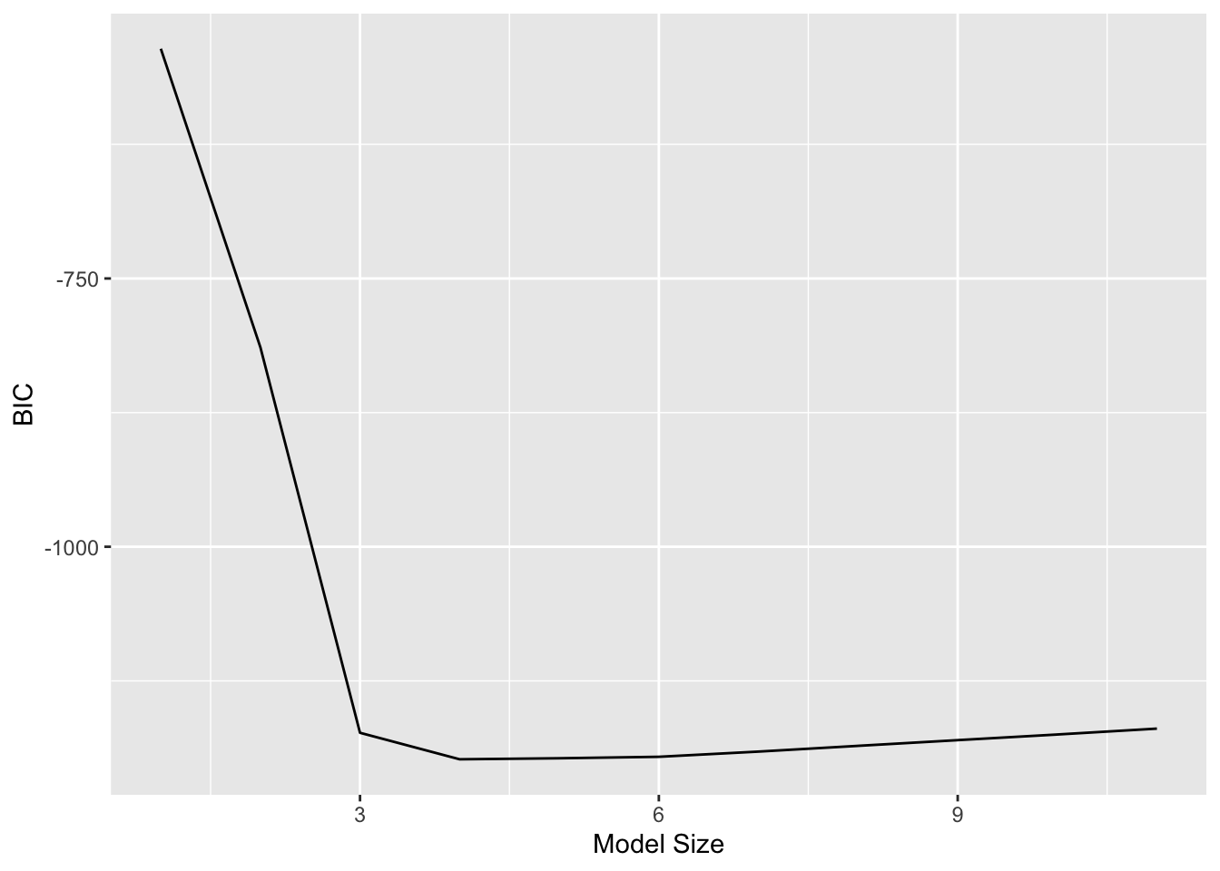
BIC chooses the best model of size 4: income, limit, cards and student.
Although we have presented best subset selection here for least squares regression, the same ideas apply to other types of models, such as logistic regression (discussed in Chapter 4). The deviance (negative two times the maximized log-likelihood) plays the role of RSS for a broader class of models.
For computational reasons, best subset selection cannot be applied with very large \(p\). When \(p = 20\), there are \(2^p = 1,048,576\) models!
Stepwise methods, which explore a far more restricted set of models, are attractive alternatives to best subset selection.
3.2 Forward stepwise selection
Forward stepwise selection begins with a model containing no predictors, and then adds predictors to the model, one-at-a-time, until all of the predictors are in the model.
In particular, at each step the variable that gives the greatest additional improvement to the fit is added to the model.
Forward stepwise selection algorithm:
Let \(\mathcal{M}_0\) be the null model, which contains no predictors besides the intercept.
For \(k = 0,1,\ldots, p-1\):
Consider all \(p-k\) models that augment the predictors in \(\mathcal{M}_k\) with one additional predictor.
Pick the best among these \(p-k\) models, and call it \(\mathcal{M}_{k+1}\). Here best is defined as having the smallest RSS, or equivalently largest \(R^2\).
Select a single best model from among \(\mathcal{M}_0, \mathcal{M}_1, \ldots, \mathcal{M}_p\) using cross-validated prediction error, \(C_p\) (AIC), BIC, or adjusted \(R^2\).
Forward stepwise selection for the Credit data.
library(leaps)# Fit best subset regressionfs_mod <-regsubsets( Balance ~ ., data = Credit, method ="forward",nvmax =11 ) %>%summary()fs_mod
Best subset and forward stepwise selections start to differ from \(\mathcal{M}_4\).
Computational advantage of forward stepwise selection over best subset selection is clear.
It is not guaranteed to find the best possible model out of all \(2^p\) models containing subsets of the \(p\) predictors.
3.3 Backward stepwise regression
Backward stepwise selection algorithm:
Let \(\mathcal{M}_0\) be the full model, which contains all \(p\) predictors.
For \(k = p,p-1,\ldots, 1\):
Consider all \(k\) models that contain all but one of the predictors in \(\mathcal{M}_k\), for a total of \(k-1\) predictors.
Pick the best among these \(k\) models, and call it \(\mathcal{M}_{k}\). Here best is defined as having the smallest RSS, or equivalently largest \(R^2\).
Select a single best model from among \(\mathcal{M}_0, \mathcal{M}_1, \ldots, \mathcal{M}_p\) using cross-validated prediction error, \(C_p\) (AIC), BIC, or adjusted \(R^2\).
library(leaps)# Fit best subset regressionbs_mod <-regsubsets( Balance ~ ., data = Credit, method ="backward",nvmax =11 ) %>%summary()bs_mod
For the Credit data, backward stepwise selection matches the best subset selection up to \(\mathcal{M}_4\) (backwards).
Like forward stepwise selection, the backward selection approach searches through only \(1 + p(p+1)/2\) models, and so can be applied in settings where \(p\) is too large to apply best subset selection. When \(p=20\), only \(1 + p(p+1)/2 = 211\) models.
Like forward stepwise selection, backward stepwise selection is not guaranteed to yield the best model containing a subset of the \(p\) predictors.
Backward selection requires that the number of samples \(n\) is larger than the number of variables \(p\) (so that the full model can be fit). In contrast, forward stepwise can be used even when \(n < p\), and so is the only viable subset method when \(p\) is very large.
4 Criteria for model selection
The model containing all of the predictors will always have the smallest RSS and the largest \(R^2\), since these quantities are related to the training error.
We wish to choose a model with low test error, not a model with low training error. Recall that training error is usually a poor estimate of test error.
Therefore, RSS and \(R^2\) are not suitable for selecting the best model among a collection of models with different numbers of predictors.
Two approaches for estimating test error:
We can indirectly estimate test error by making an adjustment to the training error to account for the bias due to overfitting.
We can directly estimate the test error, using either a validation set approach or a cross-validation approach, as discussed in next lectures.
Mallow’s \(C_p\): \[
C_p = \frac{1}{n} (\text{RSS} + 2d \hat{\sigma}^2),
\] where \(d\) is the total number of parameters used and \(\hat{\sigma}^2\) is an estimate of the error variance \(\text{Var}(\epsilon)\). Smaller \(C_p\) means better model.
The AIC criterion: \[
\text{AIC} = - 2 \log L + 2d,
\] where \(L\) is the maximized value of the likelihood function for the estimated model. Smaller AIC means better model.
In the case of the linear model with Gaussian errors, maximum likelihood and least squares are the same thing, and \(C_p\) and AIC are equivalent.
BIC: \[
\text{BIC} = \frac{1}{n}(\text{RSS} + \log(n) d \hat{\sigma}^2).
\] Smaller BIC means better model.
Since \(\log n > 2\) for any \(n > 7\), the BIC statistic generally places a heavier penalty on models with many variables, and hence results in the selection of smaller models than \(C_p\).
Adjusted \(R^2\): \[
\text{Adjusted } R^2 = 1 - \frac{\text{RSS}/(n - d - 1)}{\text{TSS} / (n - 1)}.
\] A large value of adjusted \(R^2\) indicates a model with a small test error.
Maximizing the adjusted \(R^2\) is equivalent to minimizing \(\text{RSS} / (n - d - 1)\).
Figure 1: \(C_p\), BIC, and adjusted \(R^2\) are shown for the best models of each size for the Credit data set. \(C_p\) and BIC are estimates of test MSE. In the middle plot we see that the BIC estimate of test error shows an increase after four variables are selected. The other two plots are rather flat after four variables are included.
\(C_p\), AIC and BIC have theoretical justification. As sample size \(n\) is very large, they are guaranteed to find the best model. Adjusted \(R^2\) is less motivated in statistical theory.
Indirect methods hold great computational advantage. They just require a single fit of the training data.
4.2 Direct approaches: validation and cross-validation
We’ll discuss validation and cross-validation (CV) in details in Chapter 5. - This procedure has an advantage relative to AIC, BIC, \(C_p\), and adjusted \(R^2\), in that it provides a direct estimate of the test error, and doesn’t require an estimate of the error variance \(\sigma^2\).
It can also be used in a wider range of model selection tasks, even in cases where it is hard to pinpoint the model degrees of freedom (e.g. the number of predictors in the model) or hard to estimate the error variance \(\sigma^2\).
Figure 2: Square root of BIC, validation set error, and CV error for the Credit data.
5 Shrinkage methods
The subset selection methods use least squares to fit a linear model that contains a subset of the predictors.
As an alternative, we can fit a model containing all \(p\) predictors using a technique that constrains or regularizes the coefficient estimates, or equivalently, that shrinks the coefficient estimates towards zero.
It may not be immediately obvious why such a constraint should improve the fit, but it turns out that shrinking the coefficient estimates can significantly reduce their variance.
5.1 Ridge regression
Recall that the least squares estimates \(\beta_0, \beta_1, \ldots, \beta_p\) using the value that minimizes \[
\text{RSS} = \sum_{i=1}^n \left( y_i - \beta_0 - \sum_{j=1}^p \beta_j x_{ij} \right)^2.
\]
In contrast, the ridge regression coefficient estimates \(\hat{\beta}^R\) are the values that minimize \[
\text{RSS} + \lambda \sum_{j=1}^p \beta_j^2,
\] where \(\lambda \ge 0\) is a tuning parameter, to be determined separately.
Similar to least squares, ridge regression seeks coefficient estimates that fit the data well, by making the RSS small.
However, the second term, \(\lambda \sum_{j} \beta_j^2\), called a shrinkage penalty, is small when \(\beta_1, \ldots, \beta_p\) are close to zero, and so it has the effect of shrinking the estimates of \(\beta_j\) towards zero.
Since scikit-learn only takes arrays \(X\) and \(y\), we first apply transformers to transform the dataframe Credit into arrays.
There are two ways to treat dummy coding of of categorical variables: standardize or not. For consistency with ISL textbook, we standardize dummy coding here:
from sklearn.preprocessing import OneHotEncoder, StandardScalerfrom sklearn.compose import make_column_transformerfrom sklearn.pipeline import Pipeline# Response vectory = Credit.Balance# Dummy encoding for categorical variablescattr = make_column_transformer( (OneHotEncoder(drop ='first'), ['Own', 'Student', 'Married', 'Region']), remainder ='passthrough')# Standardization for ALL variables including dummy coding# Note the order of columns changed (dummy coding go first)pipe = Pipeline([('cat_tf', cattr), ('std_tf', StandardScaler())])X = pipe.fit_transform(Credit.drop('Balance', axis =1))X.shape
(400, 11)
Alternatively (and preferred), we don’t standardize dummy coding for categorical variables.
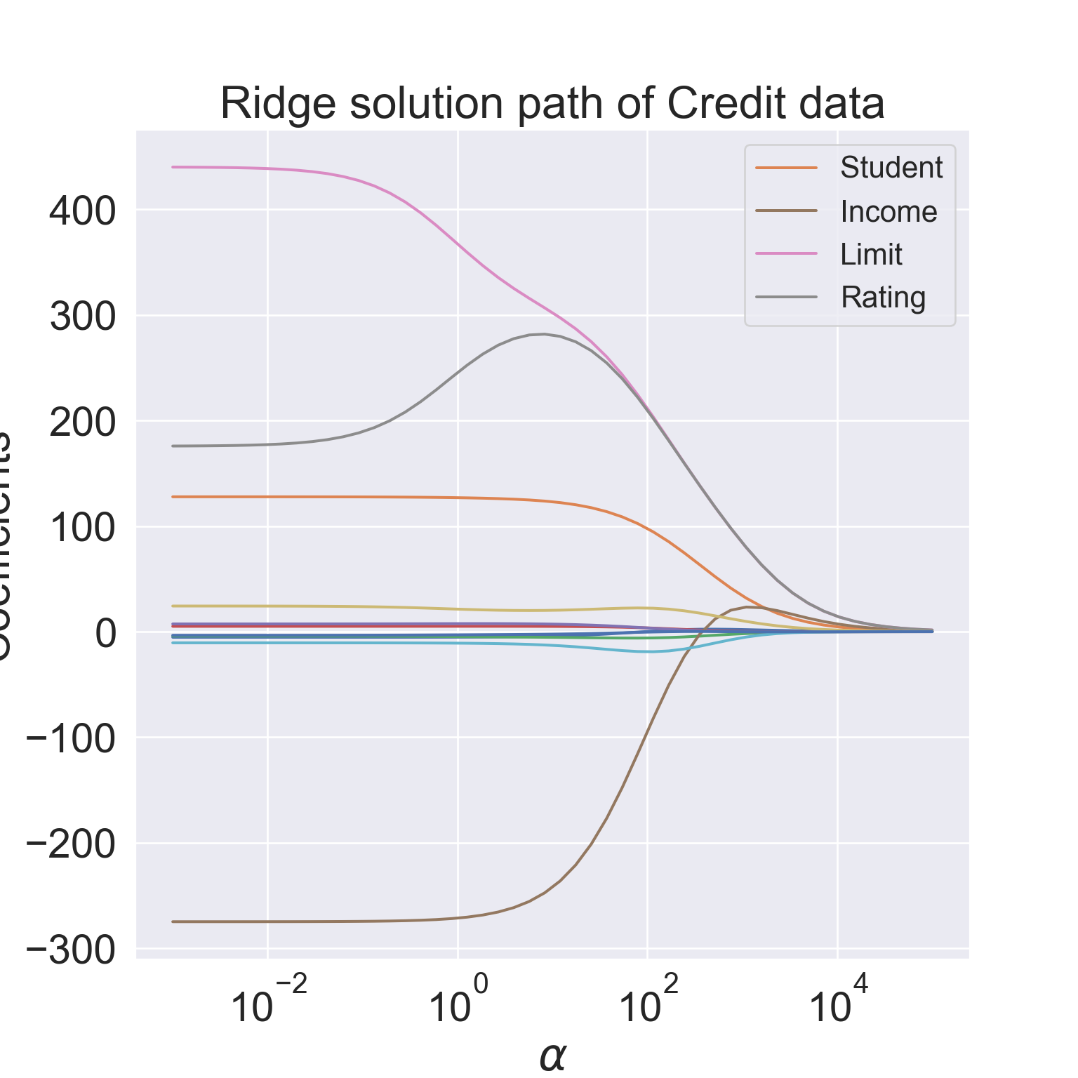
Fit ridge regression at a grid of tuning/regularization parameter values. Note the regularization parameter in the ridge regression in scikit-learn is called \(\alpha\).
from sklearn.linear_model import Ridgeclf = Ridge()# Ridge regularization parameteralphas = np.logspace(start =-3, stop =5, base =10)# Train the model with different regularization strengthscoefs = []for a in alphas: clf.set_params(alpha = a) clf.fit(X, y) coefs.append(clf.coef_)
Ridge(alpha=100000.0)
In a Jupyter environment, please rerun this cell to show the HTML representation or trust the notebook. On GitHub, the HTML representation is unable to render, please try loading this page with nbviewer.org.
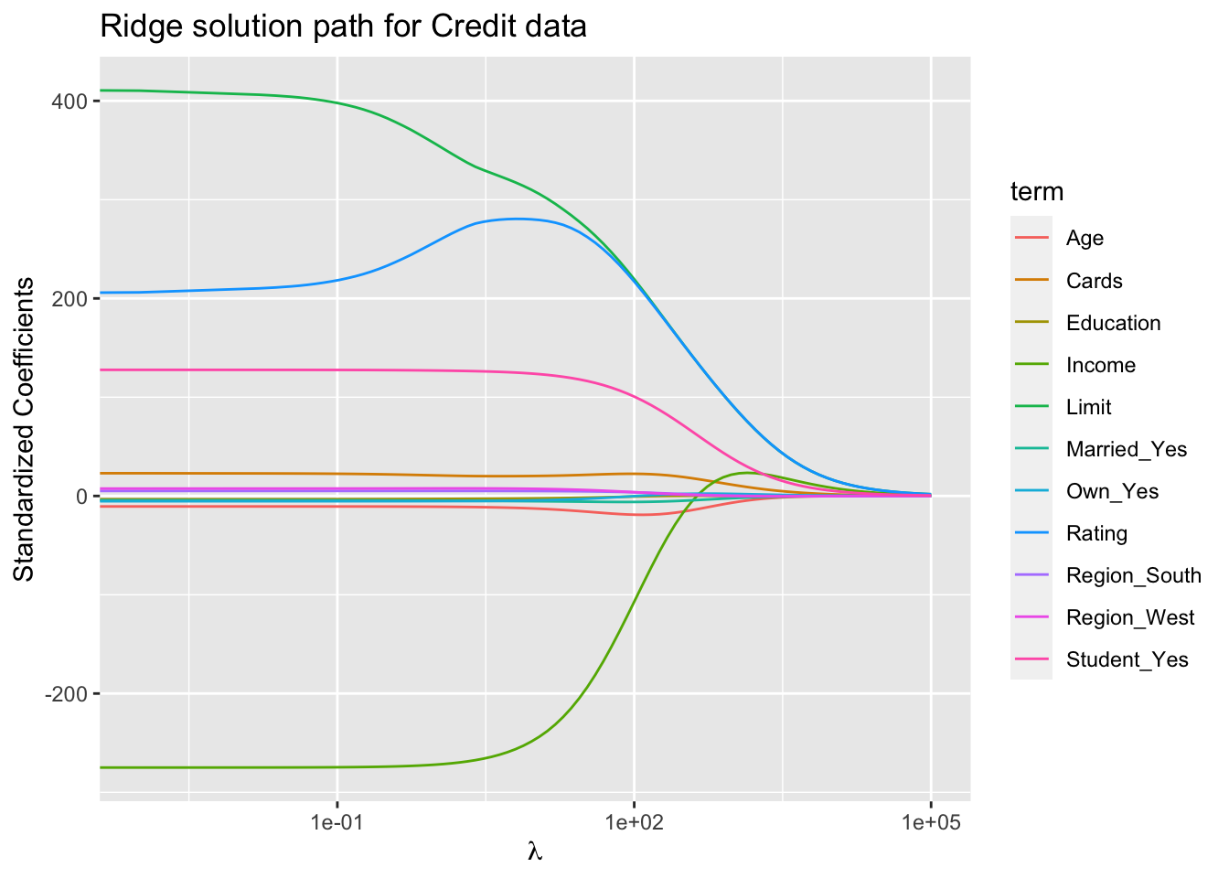
library(tidymodels)norm_recipe <-recipe( Balance ~ ., data = Credit ) %>%# create traditional dummy variablesstep_dummy(all_nominal()) %>%# zero-variance filterstep_zv(all_predictors()) %>%# center and scale numeric datastep_normalize(all_predictors()) %>%# step_log(Salary, base = 10) %>%# estimate the means and standard deviationsprep(training = Credit, retain =TRUE)norm_recipe
Recipe

Inputs:

      role #variables
   outcome          1
 predictor         10

Training data contained 400 data points and no missing data.

Operations:

Dummy variables from Own, Student, Married, Region [trained]
Zero variance filter removed <none> [trained]
Centering and scaling for Income, Limit, Rating, Cards, Age, Education, O... [trained]
Warning: Transformation introduced infinite values in continuous x-axis
Figure 3: Ridge solution path for the Credit data (ISL2 Figure 6.4).
The standard least squares coefficient estimates are scale equivariant: multiplying \(X_j\) by a constant \(c\) simply leads to a scaling of the least squares coefficient estimates by a factor of \(1/c\). In other words, regardless of how the \(j\)th predictor is scaled, \(X_j \hat{\beta}_j\) will remain the same.
In contrast, the ridge regression coefficient estimates can change substantially when multiplying a given predictor by a constant, due to the sum of squared coefficients term in the penalty part of the ridge regression objective function.
Therefore, it is best to apply ridge regression after standardizing the predictors, using the formula \[
\tilde{x}_{ij} = \frac{x_{ij}}{\sqrt{\frac{1}{n} \sum_{i=1}^n (x_{ij} - \bar{x}_j)^2}}.
\]
Why Does Ridge Regression Improve Over Least Squares? Answer: the bias-variance tradeoff.
Figure 4: Simulated data with \(n = 50\) observations, \(p = 45\) predictors, all having nonzero coefficients. Squared bias (black), variance (green), and test mean squared error (purple) for the ridge regression predictions on a simulated data set, as a function of \(\lambda\) and \(\|\hat{\beta}_{\lambda}^R\|_2 / \|\hat{\beta}\|_2\). The horizontal dashed lines indicate the minimum possible MSE. The purple crosses indicate the ridge regression models for which the test MSE is smallest.
The tuning parameter \(\lambda\) serves to control the relative impact of these two terms on the regression coefficient estimates.
Selecting a good value for \(\lambda\) is critical. Cross-validation can be used for this.
5.2 Lasso
Ridge regression does have one obvious disadvantage: unlike subset selections, which will generally select models that involve just a subset of the variables, ridge regression will include all \(p\) predictors in the final model.
Lasso is a relatively recent alternative to ridge regression that overcomes this disadvantage. The lasso coefficients, \(\hat{\beta}_\lambda^L\), minimize the quantity \[
\text{RSS} + \lambda \sum_{j=1}^p |\beta_j|.
\]
In statistical parlance, the lasso uses an \(\ell_1\) (pronounced “ell 1”) penalty instead of an \(\ell_2\) penalty. The \(\ell_1\) norm of a coefficient vector \(\beta\) is given by \(\|\beta\|_1 = \sum_j |\beta_j|\).
As with ridge regression, the lasso shrinks the coefficient estimates towards zero.
However, in the case of the lasso, the \(\ell_1\) penalty has the effect of forcing some of the coefficient estimates to be exactly equal to zero when the tuning parameter \(\lambda\) is sufficiently large.
Hence, much like best subset selection, the lasso performs variable selection.
We say that the lasso yields sparse models. The models involve only a subset of the variables.
As in ridge regression, selecting a good value of \(\lambda\) for the lasso is critical. Cross-validation is again the method of choice.
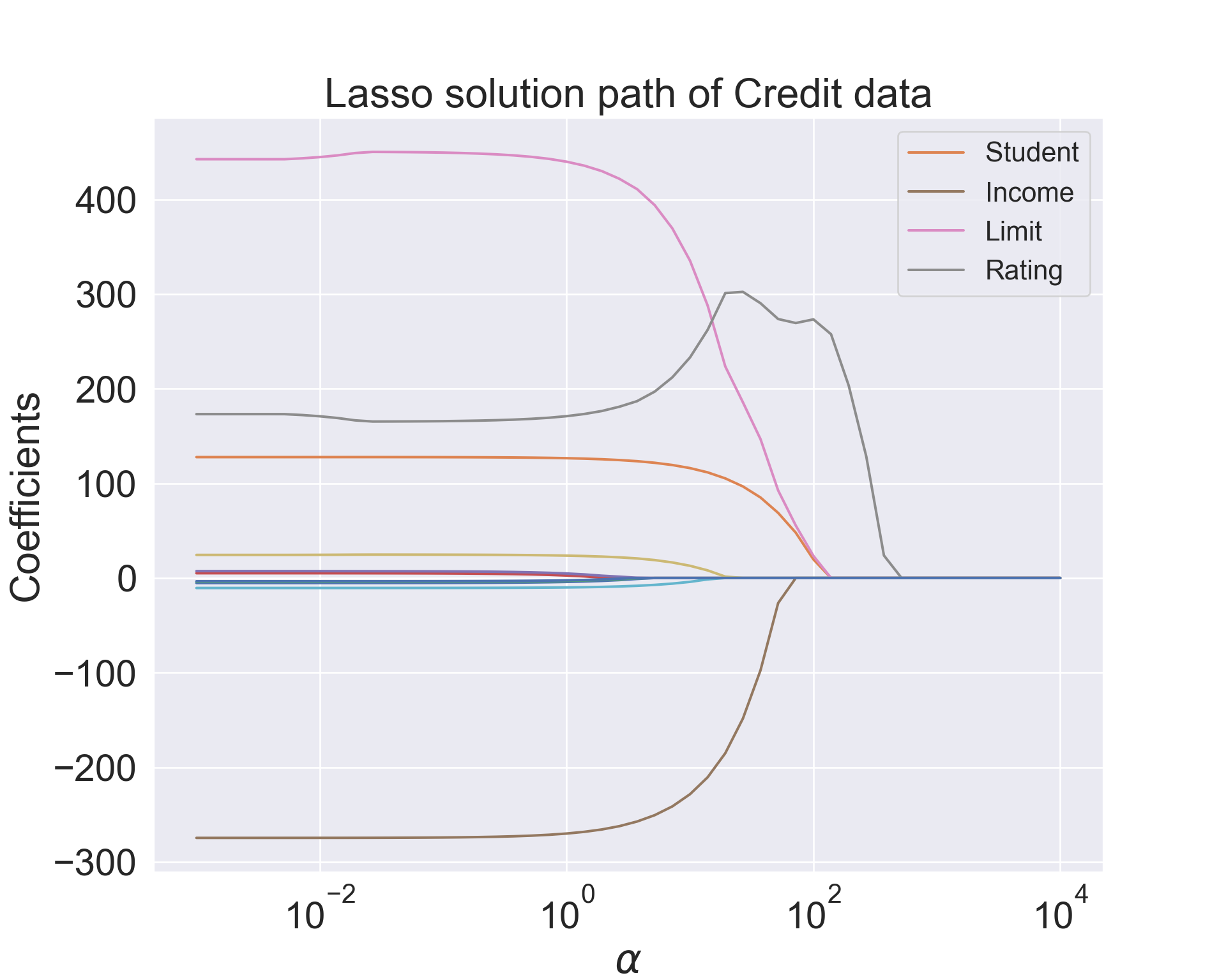
from sklearn.linear_model import Lassoclf = Lasso()# Ridge regularization parameteralphas = np.logspace(start =-3, stop =4, base =10)# Train the model with different regularization strengthscoefs = []for a in alphas: clf.set_params(alpha = a) clf.fit(X, y) coefs.append(clf.coef_)
Lasso(alpha=10000.0)
In a Jupyter environment, please rerun this cell to show the HTML representation or trust the notebook. On GitHub, the HTML representation is unable to render, please try loading this page with nbviewer.org.
Warning: Transformation introduced infinite values in continuous x-axis
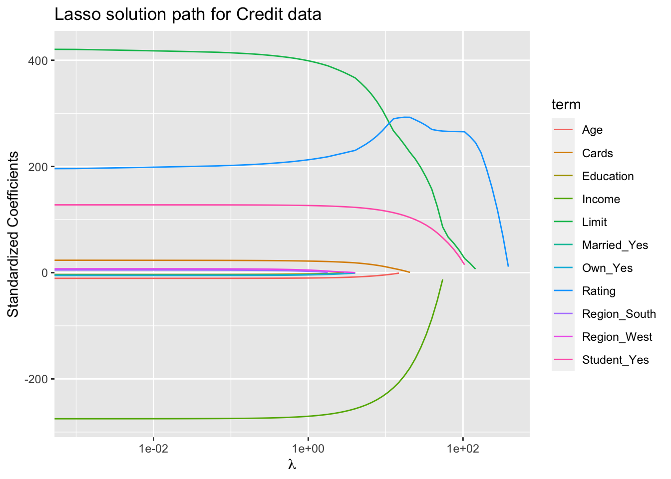
Figure 5: Lasso solution path for the Credit data (ISL Figure 6.6).
Why is it that the lasso, unlike ridge regression, results in coefficient estimates that are exactly equal to zero?
One can show that the lasso and ridge regression coefficient estimates solve the problems \[
\text{minimize } \text{RSS} \quad \text{ subject to } \sum_{j=1}^p |\beta_j| \le s
\] and \[
\text{minimize } \text{RSS} \quad \text{ subject to } \sum_{j=1}^p \beta_j^2 \le s
\] respectively.
Figure 6: Contours of the RSS and constraint functions for the lasso (left) and ridge regression (right). The solid blue areas are the constraint regions, \(|\beta_1| + |\beta_2| \le s\) and \(\beta_1^2 + \beta_2^2 \le s\), while the red ellipses are the contours of the RSS.
5.3 Comparing ridge and lasso
Simulation example with \(n=50\) and \(p=45\). All 45 predictors are related to response.
Figure 7: Left: Plots of squared bias (black), variance (green), and test MSE (purple) for the lasso. Right: Comparison of squared bias, variance and test MSE between lasso (solid) and ridge (dashed). Both are plotted against their \(R^2\) on the training data, as a common form of indexing. The crosses in both plots indicate the lasso model for which the MSE is smallest.
Simulation example with \(n=50\) and \(p=45\). Only 2 predictors are related to response.
Figure 8: Left: Plots of squared bias (black), variance (green), and test MSE (purple) for the lasso. The simulated data is similar, except that now only two predictors are related to the response. Right: Comparison of squared bias, variance and test MSE between lasso (solid) and ridge (dashed). Both are plotted against their \(R^2\) on the training data, as a common form of indexing. The crosses in both plots indicate the lasso model for which the MSE is smallest.
These two examples illustrate that neither ridge regression nor the lasso will universally dominate the other.
In general, one might expect the lasso to perform better when the response is a function of only a relatively small number of predictors.
However, the number of predictors that is related to the response is never known a priori for real data sets.
A technique such as cross-validation can be used in order to determine which approach is better on a particular data set.
5.4 Selecting the tuning parameter for ridge regression and lasso
Similar to subset selection, for ridge regression and lasso we require a method to determine which of the models under consideration is best.
That is, we require a method selecting a value for the tuning parameter \(\lambda\) or equivalently, the value of the constraint \(s\).
Cross-validation provides a simple way to tackle this problem. We choose a grid of \(\lambda\) values, and compute the cross-validation error rate for each value of \(\lambda\).
We then select the tuning parameter value for which the cross-validation error is smallest.
Finally, the model is re-fit using all of the available observations and the selected value of the tuning parameter.
Figure 9: Left: Cross-validation errors that result from applying ridge regression to the Credit data set with various values of \(\lambda\). Right: The coefficient estimates as a function of \(\lambda\). The vertical dashed lines indicate the value of \(\lambda\) selected by cross-validation. (ISL Figure 6.12)
6 Dimension reduction methods
The methods that we have discussed so far have involved fitting linear regression models, via least squares or a shrunken approach, using the original predictors, \(X_1, X_2, \ldots, X_p\).
We now explore a class of approaches that transform the predictors and then fit a least squares model using the transformed variables. We will refer to these techniques as dimension reduction methods.
Let \(Z_1, Z_2, \ldots, Z_M\) represent \(M < p\)linear combinations of our original \(p\) predictors. That is \[
Z_m = \sum_{j=1}^p \phi_{mj} X_j
\tag{1}\] for some constants \(\phi_{m1}, \ldots, \phi_{mp}\).
We can then fit the linear regression model, \[
y_i = \theta_0 + \sum_{m=1}^M \theta_m z_{im} + \epsilon_i, \quad i = 1,\ldots,n,
\tag{2}\] using ordinary least squares. Here \(\theta_0, \theta_1, \ldots, \theta_M\) are the regression coefficients.
Hence model Equation 2 can be thought of as a special case of the original linear regression model.
Dimension reduction serves to constrain the estimated \(\beta_j\) coefficients, since now they must take the form Equation 3.
Can win in the bias-variance tradeoff.
6.1 Principal components regression
Principal components regression (PCR) applies principal components analysis (PCA) to define the linear combinations of the predictors, for use in our regression.
The first principal component \(Z_1\) is the (normalized) linear combination of the variables with the largest variance.
The second principal component \(Z_2\) has largest variance, subject to being uncorrelated with the first.
And so on.
Hence with many correlated original variables, we replace them with a small set of principal components that capture their joint variation.
Figure 10: The population size (pop) and ad spending (ad) for 100 different cities are shown as purple circles. The green solid line indicates the first principal component, and the blue dashed line indicates the second principal component.
The first principal component \[
Z_1 = 0.839 \times (\text{pop} - \bar{\text{pop}}) + 0.544 \times (\text{ad} - \bar{\text{ad}}).
\]
Out of all possible linear combination of pop and ad such that \(\phi_{11}^2 + \phi_{21}^2 = 1\) (why do we need this constraint?), this particular combination yields the highest variance.
There is also another interpretation for PCA: the first principal component vector defines the line that is as close as possible to the data.
Figure 11: A subset of the advertising data. Left: The first principal component, chosen to minimize the sum of the squared perpendicular distances to each point, is shown in green. These distances are represented using the black dashed line segments. Right: The left-hand panel has been rotated so that the first principal component lies on the \(x\)-axis.
The first principal component appears to capture most of the information contained in the pop and ad predictors.
Figure 12: Plots of the first principal component scores \(z_{i1}\) versus pop and ad. The relationships are strong.
The second principal component \[
Z_2 = 0.544 \times (\text{pop} - \bar{\text{pop}}) - 0.839 \times (\text{ad} - \bar{\text{ad}}).
\]
Figure 13: Plots of the second principal component scores \(z_{i2}\) versus pop and ad. The relationships are weak.
PCR applied to two simulation data sets with \(n=50\) and \(p=45\):
Figure 14: PCR was applied to two simulated data sets. The black, green, and purple lines correspond to squared bias, variance, and test mean squared error, respectively. Left: all 45 predictors are related to response. Right: Only 2 out of 45 predictors are related to response.
PCR applied to a data set where the first 5 principal components are related to response.
Figure 15: PCR, ridge regression, and the lasso were applied to a simulated data set in which the first five principal components of \(X\) contain all the information about the response \(Y\). In each panel, the irreducible error \(\operatorname{Var}(\epsilon)\) is shown as a horizontal dashed line. Left: Results for PCR. Right: Results for lasso (solid) and ridge regression (dotted). The \(x\)-axis displays the shrinkage factor of the coefficient estimates, defined as the \(\ell_2\) norm of the shrunken coefficient estimates divided by the \(\ell_2\) norm of the least squares estimate.
PCR applied to the Credit data:
Figure 16: PCR was applied to the Credit data.
6.2 Partial least squares (PLS)
PCR identifies linear combinations, or directions, that best represent the predictors \(X_1, \ldots, X_p\).
These directions are identified in an unsupervised way, since the response \(Y\) is not used to help determine the principal component directions.
That is, the response does not supervise the identification of the principal components.
Consequently, PCR suffers from a potentially serious drawback: there is no guarantee that the directions that best explain the predictors will also be the best directions to use for predicting the response.
Like PCR, partial least squares (PLS) is a dimension reduction method, which first identifies a new set of features \(Z_1, \ldots, Z_M\) that are linear combinations of the original features, and then fits a linear model via OLS using these \(M\) new features.
But unlike PCR, PLS identifies these new features in a supervised way. That is it makes use of the response \(Y\) in order to identify new features that not only approximate the old features well, but also that are related to the response.
Roughly speaking, the PLS approach attempts to find directions that help explain both the response and the predictors.
PLS algorithm:
After standardizing the \(p\) predictors, PLS computes the first direction \(Z_1\) by setting each \(\phi_{1j}\) in Equation 1 equal to the coefficient from the simple linear regression of \(Y\) onto \(X_j\).
One can show that this coefficient is proportional to the correlation between \(Y\) and \(X_j\).
Hence, in computing \(Z_1 = \sum_{j=1}^p \phi_{1j} X_j\), PLS places the highest weight on the variables that are most strongly related to the response.
Subsequent directions are found by taking residuals and then repeating the above procedure.
7 Summary
Model selection methods are an essential tool for data analysis, especially for big datasets involving many predictors.
Research into methods that give sparsity, such as the lasso is an especially hot area.
Later, we will return to sparsity in more detail, and will describe related approaches such as the elastic net.