Machine Learning Workflow: Boosting for Prediction

Econ 425T

Display system information for reproducibility.

Python

import IPython
print(IPython.sys_info())

{'commit_hash': 'add5877a4',
 'commit_source': 'installation',
 'default_encoding': 'utf-8',
 'ipython_path': '/Library/Frameworks/Python.framework/Versions/3.10/lib/python3.10/site-packages/IPython',
 'ipython_version': '8.8.0',
 'os_name': 'posix',
 'platform': 'macOS-10.16-x86_64-i386-64bit',
 'sys_executable': '/Library/Frameworks/Python.framework/Versions/3.10/bin/python3',
 'sys_platform': 'darwin',
 'sys_version': '3.10.9 (v3.10.9:1dd9be6584, Dec  6 2022, 14:37:36) [Clang '
                '13.0.0 (clang-1300.0.29.30)]'}

1 Overview

We illustrate the typical machine learning workflow for random forests using the Hitters data set from R ISLR2 package.

1. Initial splitting to test and non-test sets.

2. Pre-processing of data: not much is needed for regression trees.

3. Tune the cost complexity pruning hyper-parameter(s) using 10-fold cross-validation (CV) on the non-test data.

4. Choose the best model by CV and refit it on the whole non-test data.

5. Final prediction on the test data.

2 Hitters data

A documentation of the Hitters data is here. The goal is to predict the log(Salary) (at opening of 1987 season) of MLB players from their performance metrics in the 1986-7 season.

Python

# Load the pandas library
import pandas as pd
# Load numpy for array manipulation
import numpy as np
# Load seaborn plotting library
import seaborn as sns
import matplotlib.pyplot as plt

# Set font sizes in plots
sns.set(font_scale = 1.2)
# Display all columns
pd.set_option('display.max_columns', None)

Hitters = pd.read_csv("../data/Hitters.csv")
Hitters

     AtBat  Hits  HmRun  Runs  RBI  Walks  Years  CAtBat  CHits  CHmRun  \
0      293    66      1    30   29     14      1     293     66       1   
1      315    81      7    24   38     39     14    3449    835      69   
2      479   130     18    66   72     76      3    1624    457      63   
3      496   141     20    65   78     37     11    5628   1575     225   
4      321    87     10    39   42     30      2     396    101      12   
..     ...   ...    ...   ...  ...    ...    ...     ...    ...     ...   
317    497   127      7    65   48     37      5    2703    806      32   
318    492   136      5    76   50     94     12    5511   1511      39   
319    475   126      3    61   43     52      6    1700    433       7   
320    573   144      9    85   60     78      8    3198    857      97   
321    631   170      9    77   44     31     11    4908   1457      30   

     CRuns  CRBI  CWalks League Division  PutOuts  Assists  Errors  Salary  \
0       30    29      14      A        E      446       33      20     NaN   
1      321   414     375      N        W      632       43      10   475.0   
2      224   266     263      A        W      880       82      14   480.0   
3      828   838     354      N        E      200       11       3   500.0   
4       48    46      33      N        E      805       40       4    91.5   
..     ...   ...     ...    ...      ...      ...      ...     ...     ...   
317    379   311     138      N        E      325        9       3   700.0   
318    897   451     875      A        E      313      381      20   875.0   
319    217    93     146      A        W       37      113       7   385.0   
320    470   420     332      A        E     1314      131      12   960.0   
321    775   357     249      A        W      408        4       3  1000.0   

    NewLeague  
0           A  
1           N  
2           A  
3           N  
4           N  
..        ...  
317         N  
318         A  
319         A  
320         A  
321         A  

[322 rows x 20 columns]

# Numerical summaries
Hitters.describe()

            AtBat        Hits       HmRun        Runs         RBI       Walks  \
count  322.000000  322.000000  322.000000  322.000000  322.000000  322.000000   
mean   380.928571  101.024845   10.770186   50.909938   48.027950   38.742236   
std    153.404981   46.454741    8.709037   26.024095   26.166895   21.639327   
min     16.000000    1.000000    0.000000    0.000000    0.000000    0.000000   
25%    255.250000   64.000000    4.000000   30.250000   28.000000   22.000000   
50%    379.500000   96.000000    8.000000   48.000000   44.000000   35.000000   
75%    512.000000  137.000000   16.000000   69.000000   64.750000   53.000000   
max    687.000000  238.000000   40.000000  130.000000  121.000000  105.000000   

            Years       CAtBat        CHits      CHmRun        CRuns  \
count  322.000000    322.00000   322.000000  322.000000   322.000000   
mean     7.444099   2648.68323   717.571429   69.490683   358.795031   
std      4.926087   2324.20587   654.472627   86.266061   334.105886   
min      1.000000     19.00000     4.000000    0.000000     1.000000   
25%      4.000000    816.75000   209.000000   14.000000   100.250000   
50%      6.000000   1928.00000   508.000000   37.500000   247.000000   
75%     11.000000   3924.25000  1059.250000   90.000000   526.250000   
max     24.000000  14053.00000  4256.000000  548.000000  2165.000000   

              CRBI       CWalks      PutOuts     Assists      Errors  \
count   322.000000   322.000000   322.000000  322.000000  322.000000   
mean    330.118012   260.239130   288.937888  106.913043    8.040373   
std     333.219617   267.058085   280.704614  136.854876    6.368359   
min       0.000000     0.000000     0.000000    0.000000    0.000000   
25%      88.750000    67.250000   109.250000    7.000000    3.000000   
50%     220.500000   170.500000   212.000000   39.500000    6.000000   
75%     426.250000   339.250000   325.000000  166.000000   11.000000   
max    1659.000000  1566.000000  1378.000000  492.000000   32.000000   

            Salary  
count   263.000000  
mean    535.925882  
std     451.118681  
min      67.500000  
25%     190.000000  
50%     425.000000  
75%     750.000000  
max    2460.000000  

Graphical summary:

# Graphical summaries
plt.figure()
sns.pairplot(data = Hitters);
plt.show()

There are 59 NAs for the salary. Let’s drop those cases. We are left with 263 data points.

Hitters.dropna(inplace = True)
Hitters.shape

(263, 20)

3 Initial split into test and non-test sets

We randomly split the data in half of test data and another half of non-test data.

Python

from sklearn.model_selection import train_test_split

Hitters_other, Hitters_test = train_test_split(
  Hitters, 
  train_size = 0.5,
  random_state = 425, # seed
  )
Hitters_test.shape

(132, 20)

Hitters_other.shape

(131, 20)

Separate \(X\) and \(y\). We will use 9 of the features.

features = ['Assists', 'AtBat', 'Hits', 'HmRun', 'PutOuts', 'RBI', 'Runs', 'Walks', 'Years']
# Non-test X and y
X_other = Hitters_other[features]
y_other = np.log(Hitters_other.Salary)
# Test X and y
X_test = Hitters_test[features]
y_test = np.log(Hitters_test.Salary)

R

4 Preprocessing (Python) or recipe (R)

Python

Not much preprocessing is needed here since all predictors are quantitative.

R

5 Model

Python

from sklearn.ensemble import AdaBoostRegressor
from sklearn.tree import DecisionTreeRegressor

bst_mod =  AdaBoostRegressor(
  # Default base estimator is DecisionTreeRegressor with max_depth = 3
  estimator = DecisionTreeRegressor(max_depth = 3),
  # Number of trees (to be tuned)
  n_estimators = 50, 
  # Learning rate (to be tuned)
  learning_rate = 1.0,
  random_state = 425
  )

R

6 Pipeline (Python) or workflow (R)

Here we bundle the preprocessing step (Python) or recipe (R) and model.

Python

from sklearn.pipeline import Pipeline

pipe = Pipeline(steps = [
  ("model", bst_mod)
  ])
pipe

Pipeline(steps=[('model',
                 AdaBoostRegressor(estimator=DecisionTreeRegressor(max_depth=3),
                                   random_state=425))])

In a Jupyter environment, please rerun this cell to show the HTML representation or trust the notebook.
On GitHub, the HTML representation is unable to render, please try loading this page with nbviewer.org.

R

7 Tuning grid

Here we tune the number of trees n_estimators and the learning rate learning_rate.

Python

# Tune hyper-parameter(s)
d_grid = [
  DecisionTreeRegressor(max_depth = 1),
  DecisionTreeRegressor(max_depth = 2),
  DecisionTreeRegressor(max_depth = 3),
  DecisionTreeRegressor(max_depth = 4)
  ]
B_grid = [50, 100, 150, 200, 250, 300, 350, 400]
lambda_grid = [0.2, 0.4, 0.6, 0.8, 1.0]
tuned_parameters = {
  "model__estimator": d_grid,
  "model__n_estimators": B_grid,
  "model__learning_rate": lambda_grid
  }
tuned_parameters  

{'model__estimator': [DecisionTreeRegressor(max_depth=1), DecisionTreeRegressor(max_depth=2), DecisionTreeRegressor(max_depth=3), DecisionTreeRegressor(max_depth=4)], 'model__n_estimators': [50, 100, 150, 200, 250, 300, 350, 400], 'model__learning_rate': [0.2, 0.4, 0.6, 0.8, 1.0]}

R

8 Cross-validation (CV)

Python

Set up CV partitions and CV criterion.

from sklearn.model_selection import GridSearchCV

# Set up CV
n_folds = 6
search = GridSearchCV(
  pipe,
  tuned_parameters,
  cv = n_folds, 
  scoring = "neg_root_mean_squared_error",
  # Refit the best model on the whole data set
  refit = True
  )

Fit CV. This is typically the most time-consuming step.

# Fit CV
search.fit(X_other, y_other)

GridSearchCV(cv=6,
             estimator=Pipeline(steps=[('model',
                                        AdaBoostRegressor(estimator=DecisionTreeRegressor(max_depth=3),
                                                          random_state=425))]),
             param_grid={'model__estimator': [DecisionTreeRegressor(max_depth=1),
                                              DecisionTreeRegressor(max_depth=2),
                                              DecisionTreeRegressor(max_depth=3),
                                              DecisionTreeRegressor(max_depth=4)],
                         'model__learning_rate': [0.2, 0.4, 0.6, 0.8, 1.0],
                         'model__n_estimators': [50, 100, 150, 200, 250, 300,
                                                 350, 400]},
             scoring='neg_root_mean_squared_error')

In a Jupyter environment, please rerun this cell to show the HTML representation or trust the notebook.
On GitHub, the HTML representation is unable to render, please try loading this page with nbviewer.org.

Visualize CV results.

Code

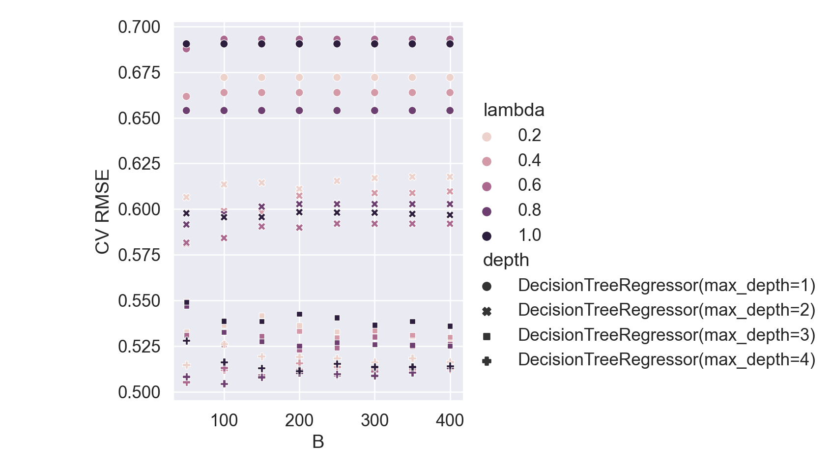
cv_res = pd.DataFrame({
  "B": np.array(search.cv_results_["param_model__n_estimators"]),
  "rmse": -search.cv_results_["mean_test_score"],
  "lambda": search.cv_results_["param_model__learning_rate"],
  "depth": search.cv_results_["param_model__estimator"],
  })

plt.figure()
sns.relplot(
  # kind = "line",
  data = cv_res,
  x = "B",
  y = "rmse",
  hue = "lambda",
  style = "depth"
  ).set(
    xlabel = "B",
    ylabel = "CV RMSE"
);
plt.show()

Best CV RMSE:

-search.best_score_

0.5043890554853537

R

9 Finalize our model

Now we are done tuning. Finally, let’s fit this final model to the whole training data and use our test data to estimate the model performance we expect to see with new data.

Python

Since we called GridSearchCV with refit = True, the best model fit on the whole non-test data is readily available.

search.best_estimator_

Pipeline(steps=[('model',
                 AdaBoostRegressor(estimator=DecisionTreeRegressor(max_depth=4),
                                   learning_rate=0.8, n_estimators=100,
                                   random_state=425))])

In a Jupyter environment, please rerun this cell to show the HTML representation or trust the notebook.
On GitHub, the HTML representation is unable to render, please try loading this page with nbviewer.org.

The final prediction RMSE on the test set is

from sklearn.metrics import mean_squared_error

mean_squared_error(
  y_test, 
  search.best_estimator_.predict(X_test), 
  squared = False
  )

0.5192563752247211

R