IMDB Sentiment Analysis (Lasso)

Econ 425T / Biostat 203B

Author

Dr. Hua Zhou @ UCLA

Published

February 23, 2023

Display system information for reproducibility.

import IPython
print(IPython.sys_info())

{'commit_hash': 'add5877a4',
 'commit_source': 'installation',
 'default_encoding': 'utf-8',
 'ipython_path': '/Users/huazhou/opt/anaconda3/lib/python3.9/site-packages/IPython',
 'ipython_version': '8.8.0',
 'os_name': 'posix',
 'platform': 'macOS-10.16-x86_64-i386-64bit',
 'sys_executable': '/Users/huazhou/opt/anaconda3/bin/python3',
 'sys_platform': 'darwin',
 'sys_version': '3.9.12 (main, Apr  5 2022, 01:56:13) \n[Clang 12.0.0 ]'}

sessionInfo()

R version 4.2.2 (2022-10-31)
Platform: x86_64-apple-darwin17.0 (64-bit)
Running under: macOS Big Sur ... 10.16

Matrix products: default
BLAS:   /Library/Frameworks/R.framework/Versions/4.2/Resources/lib/libRblas.0.dylib
LAPACK: /Library/Frameworks/R.framework/Versions/4.2/Resources/lib/libRlapack.dylib

locale:
[1] en_US.UTF-8/en_US.UTF-8/en_US.UTF-8/C/en_US.UTF-8/en_US.UTF-8

attached base packages:
[1] stats     graphics  grDevices utils     datasets  methods   base     

loaded via a namespace (and not attached):
 [1] Rcpp_1.0.9        here_1.0.1        lattice_0.20-45   png_0.1-8        
 [5] withr_2.5.0       rprojroot_2.0.3   digest_0.6.29     grid_4.2.2       
 [9] jsonlite_1.8.0    magrittr_2.0.3    evaluate_0.15     rlang_1.0.6      
[13] stringi_1.7.8     cli_3.4.1         rstudioapi_0.13   Matrix_1.5-1     
[17] reticulate_1.27   rmarkdown_2.14    tools_4.2.2       stringr_1.4.0    
[21] htmlwidgets_1.6.1 xfun_0.31         yaml_2.3.5        fastmap_1.1.0    
[25] compiler_4.2.2    htmltools_0.5.4   knitr_1.39

Load libraries.

# Load the pandas library
import pandas as pd
# Load numpy for array manipulation
import numpy as np
# Load seaborn plotting library
import seaborn as sns
import matplotlib.pyplot as plt

# Set font sizes in plots
sns.set(font_scale = 1.2)
# Display all columns
pd.set_option('display.max_columns', None)

# Load Tensorflow and Keras
import tensorflow as tf
from tensorflow import keras
from tensorflow.keras import layers

library(keras)
library(tidyverse)
library(tidymodels)
library(glmnet)
library(pROC)

1 Prepare data

From documentation:

Dataset of 25,000 movies reviews from IMDB, labeled by sentiment (positive/negative). Reviews have been preprocessed, and each review is encoded as a sequence of word indexes (integers). For convenience, words are indexed by overall frequency in the dataset, so that for instance the integer “3” encodes the 3rd most frequent word in the data. This allows for quick filtering operations such as: “only consider the top 10,000 most common words, but eliminate the top 20 most common words”.

Retrieve IMDB data. We restrict to the 10,000 most frequently-used words and tokens.

max_features = 10000

(x_train, y_train), (x_test, y_test) = keras.datasets.imdb.load_data(num_words = max_features)

Data dimensions.

x_train.shape

(25000,)

y_train.shape

(25000,)

x_test.shape

(25000,)

y_test.shape
# Indices of the first 12 words of the first training document

(25000,)

x_train[0][0:11]

[1, 14, 22, 16, 43, 530, 973, 1622, 1385, 65, 458]

To decode the reviews:

# Use the default parameters to keras.datasets.imdb.load_data
start_char = 1
oov_char = 2
index_from = 3

# Retrieve the word index file mapping words to indices
word_index = keras.datasets.imdb.get_word_index()

# Reverse the word index to obtain a dict mapping indices to words
# And add `index_from` to indices to sync with `x_train`
inverted_word_index = dict(
    (i + index_from, word) for (word, i) in word_index.items()
)

# Update `inverted_word_index` to include `start_char` and `oov_char`
inverted_word_index[start_char] = "[START]"
inverted_word_index[oov_char] = "[OOV]"
# Decode the first sequence in the dataset
" ".join(inverted_word_index[i] for i in x_train[0])

"[START] this film was just brilliant casting location scenery story direction everyone's really suited the part they played and you could just imagine being there robert [OOV] is an amazing actor and now the same being director [OOV] father came from the same scottish island as myself so i loved the fact there was a real connection with this film the witty remarks throughout the film were great it was just brilliant so much that i bought the film as soon as it was released for [OOV] and would recommend it to everyone to watch and the fly fishing was amazing really cried at the end it was so sad and you know what they say if you cry at a film it must have been good and this definitely was also [OOV] to the two little boy's that played the [OOV] of norman and paul they were just brilliant children are often left out of the [OOV] list i think because the stars that play them all grown up are such a big profile for the whole film but these children are amazing and should be praised for what they have done don't you think the whole story was so lovely because it was true and was someone's life after all that was shared with us all"

max_features <- 10000

imdb <- dataset_imdb(num_words = max_features)
x_train <- imdb$train$x
y_train <- imdb$train$y
x_test <- imdb$test$x
y_test <- imdb$test$y

Data dimensions.

# Training set
length(x_train)

[1] 25000

table(y_train)

y_train
    0     1 
12500 12500

# Test set
length(x_test)

[1] 25000

table(y_test)

y_test
    0     1 
12500 12500

# Indices of the first 12 words of the first training document
x_train[[1]][1:12]

 [1]    1   14   22   16   43  530  973 1622 1385   65  458 4468

Function for decoding the IMDB reviews:

word_index <- dataset_imdb_word_index()

decode_review <- function(text, word_index) {
  word <- names(word_index)
  idx <- unlist(word_index, use.names = FALSE)
  word <- c("<PAD>", "<START>", "<UNK>", "<UNUSED>", word)
  idx <- c(0:3, idx + 3)
  words <- word[match(text, idx, 2)]
  paste(words, collapse = " ")
}

decode_review(x_train[[1]], word_index)

[1] "<START> this film was just brilliant casting location scenery story direction everyone's really suited the part they played and you could just imagine being there robert <UNK> is an amazing actor and now the same being director <UNK> father came from the same scottish island as myself so i loved the fact there was a real connection with this film the witty remarks throughout the film were great it was just brilliant so much that i bought the film as soon as it was released for <UNK> and would recommend it to everyone to watch and the fly fishing was amazing really cried at the end it was so sad and you know what they say if you cry at a film it must have been good and this definitely was also <UNK> to the two little boy's that played the <UNK> of norman and paul they were just brilliant children are often left out of the <UNK> list i think because the stars that play them all grown up are such a big profile for the whole film but these children are amazing and should be praised for what they have done don't you think the whole story was so lovely because it was true and was someone's life after all that was shared with us all"

Create the bag of words matrices.

from scipy import sparse

def one_hot(sequences, dimension):
  seqlen = [len(sequences[i]) for i in range(len(sequences))]
  n = len(seqlen)
  rowind = np.repeat(range(n), seqlen)
  colind = np.concatenate(sequences)
  vals = np.ones(len(rowind))
  return sparse.coo_matrix((vals, (rowind, colind)), shape = (n, dimension)).tocsc()

# Train
x_train_1h = one_hot(x_train, 10000)
x_train_1h.shape
# Sparsity of train set

(25000, 10000)

x_train_1h.count_nonzero() / np.prod(x_train_1h.shape)
# Test

0.013169872

x_test_1h = one_hot(x_test, 10000)
x_test_1h.shape
# Sparsity of test set

(25000, 10000)

x_test_1h.count_nonzero() / np.prod(x_test_1h.shape)

0.012874312

library(Matrix)

one_hot <- function(sequences, dimension) {
  seqlen <- sapply(sequences, length)
  n <- length(seqlen)
  rowind <- rep(1:n, seqlen)
  colind <- unlist(sequences)
  sparseMatrix(
    i = rowind,
    j = colind,
    dims = c(n, dimension)
  )
}

# Train
x_train_1h <- one_hot(x_train, 10000)
dim(x_train_1h)

[1] 25000 10000

# Proportion of nonzeros
nnzero(x_train_1h) / (25000 * 10000)

[1] 0.01316987

# Test
x_test_1h <- one_hot(x_test, 10000)
dim(x_test_1h)

[1] 25000 10000

# Proportion of nonzeros
nnzero(x_test_1h) / (25000 * 10000)

[1] 0.01287431

2 Lasso

2.1 Training Lasso

We use logistic regression model in scikit-learn:

from sklearn.linear_model import LogisticRegression
from sklearn.pipeline import Pipeline

logit_mod = LogisticRegression(
  penalty = 'l1',
  solver = 'liblinear',
  warm_start = True
  )

pipe = Pipeline(steps = [
  ("model", logit_mod)
])
pipe

Pipeline(steps=[('model',
                 LogisticRegression(penalty='l1', solver='liblinear',
                                    warm_start=True))])

In a Jupyter environment, please rerun this cell to show the HTML representation or trust the notebook.
On GitHub, the HTML representation is unable to render, please try loading this page with nbviewer.org.

Set up tuning grid for \(C = 1/\alpha\).

C_grid = np.logspace(start = -3, stop = 3, base = 10, num = 100)

tuned_parameters = {"model__C": C_grid}

Cross-validation:

from sklearn.model_selection import GridSearchCV

# Set up CV
n_folds = 10
search = GridSearchCV(
  pipe, 
  tuned_parameters, 
  cv = n_folds, 
  scoring = "roc_auc",
  # Refit the best model on the whole data set
  refit = True,
  # Adjust n_jobs according to hardware
  n_jobs = 8
  )

search.fit(x_train_1h, y_train)

GridSearchCV(cv=10,
             estimator=Pipeline(steps=[('model',
                                        LogisticRegression(penalty='l1',
                                                           solver='liblinear',
                                                           warm_start=True))]),
             n_jobs=8,
             param_grid={'model__C': array([1.00000000e-03, 1.14975700e-03, 1.32194115e-03, 1.51991108e-03,
       1.74752840e-03, 2.00923300e-03, 2.31012970e-03, 2.65608778e-03,
       3.05385551e-03, 3.51119173e-03, 4.03701726e-03, 4.64158883e-03,
       5.3366...
       4.03701726e+01, 4.64158883e+01, 5.33669923e+01, 6.13590727e+01,
       7.05480231e+01, 8.11130831e+01, 9.32603347e+01, 1.07226722e+02,
       1.23284674e+02, 1.41747416e+02, 1.62975083e+02, 1.87381742e+02,
       2.15443469e+02, 2.47707636e+02, 2.84803587e+02, 3.27454916e+02,
       3.76493581e+02, 4.32876128e+02, 4.97702356e+02, 5.72236766e+02,
       6.57933225e+02, 7.56463328e+02, 8.69749003e+02, 1.00000000e+03])},
             scoring='roc_auc')

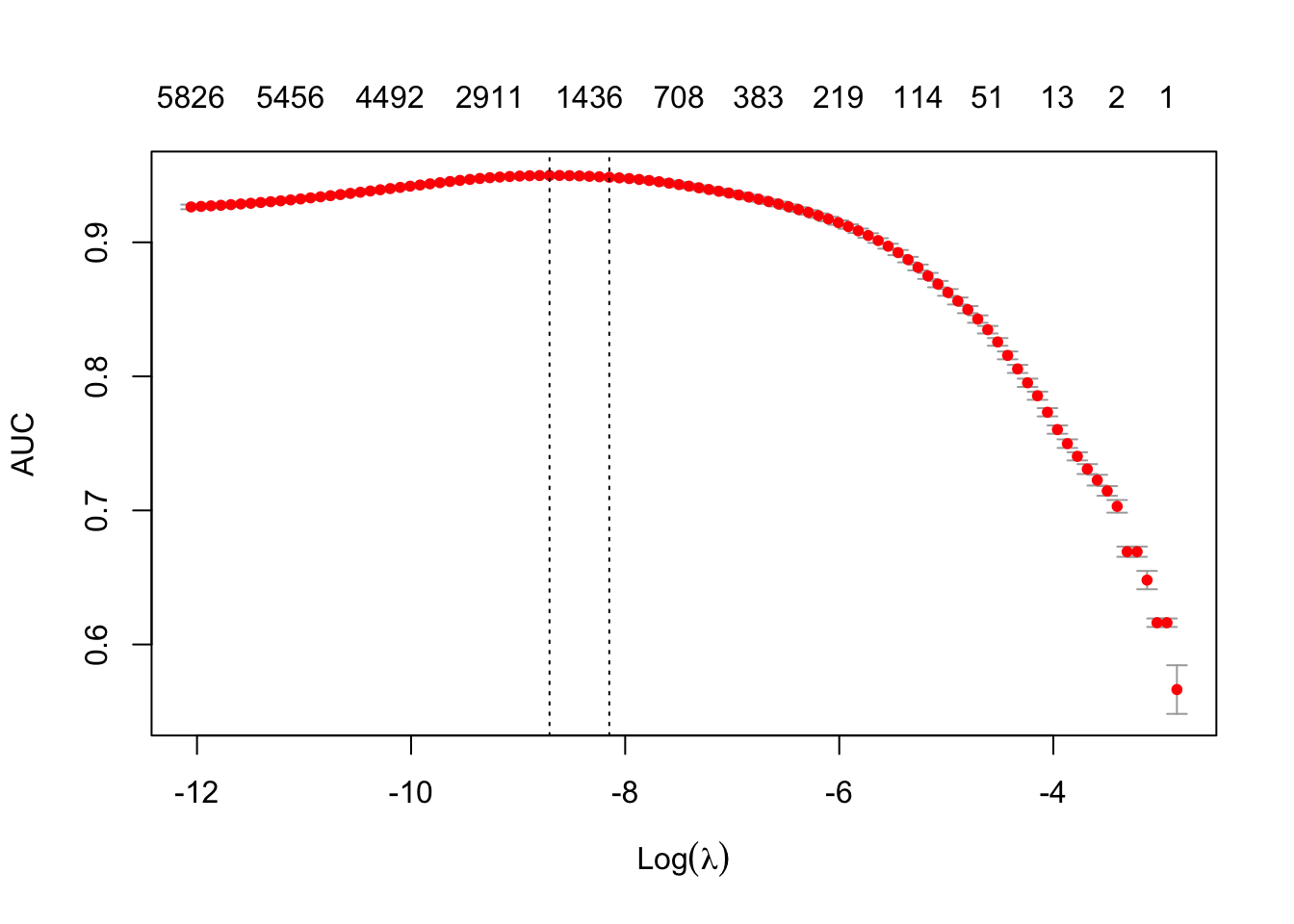
cvres <- cv.glmnet(
  x_train_1h,
  y_train,
  nfolds = 10,
  family = "binomial",
  # loss to use for CV
  type.measure = "auc",
  # pass through to glmnet
  standardize = FALSE,
)

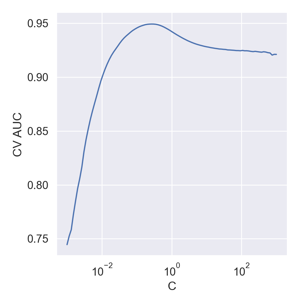
Visualize CV result:

cvres = pd.DataFrame(
  {
  "C": np.array(search.cv_results_["param_model__C"]),
  "aucroc": search.cv_results_["mean_test_score"]
  }
)

plt.figure()
sns.relplot(
  kind = "line",
  data = cvres,
  x = "C",
  y = "aucroc"
  ).set(
    xscale = "log",
    xlabel = "C",
    ylabel = "CV AUC"
);
plt.show()

plot(cvres)

Which words have the largest effect sizes in the lasso penalized logistic regression?

search.best_estimator_['model']

LogisticRegression(C=0.26560877829466867, penalty='l1', solver='liblinear',
                   warm_start=True)

betahat = search.best_estimator_['model'].coef_[0]
ix = np.argsort(abs(betahat))[::-1]

pd.DataFrame({
  'word': [inverted_word_index[i + 1 + index_from] for i in ix[range(10)]],
  'beta': betahat[ix[range(10)]]
})

           word      beta
0  entertaining -1.757356
1     developed -1.641616
2     structure  1.614953
3      surprise -1.556535
4           fun -1.513903
5          knew  1.304302
6            40  1.277682
7             v -1.268676
8      remember -1.214610
9        angles -1.204298

betahat_sorted <- sort(
  as.vector(abs(coef(cvres))), 
  decreasing = TRUE, 
  index.return = TRUE
  )

tibble(
  word = str_split(decode_review(betahat_sorted$ix[1:10], word_index), ' ')[[1]],
  beta = coef(cvres)[betahat_sorted$ix[1:10]]
)

# A tibble: 10 × 2
   word        beta
   <chr>      <dbl>
 1 cinema     -1.63
 2 girl       -1.60
 3 knows       1.35
 4 premise    -1.31
 5 loves      -1.27
 6 video      -1.24
 7 opposite   -1.14
 8 australian  1.10
 9 necessary   1.09
10 nearly     -1.09

2.2 Testing Lasso

Test AUC:

from sklearn.metrics import accuracy_score, roc_auc_score

roc_auc_score(
  y_test, 
  search.best_estimator_.predict_proba(x_test_1h)[:, 1]
  )

0.9482195072000001

Test accuracy:

accuracy_score(
  y_test,
  search.best_estimator_.predict(x_test_1h)
  )

0.8814

Test AUC:

auc(y_test, predict(cvres, x_test_1h, type = "response"))

Warning in roc.default(response, predictor, auc = TRUE, ...): Deprecated use a
matrix as predictor. Unexpected results may be produced, please pass a numeric
vector.

Area under the curve: 0.9486

Test accuracy:

sum(y_test == predict(cvres, x_test_1h, type = "class")) / length(y_test)

[1] 0.881