This example tries to reproduce the two-layer MLP for classifying IMDB reviews based on bags-of-words.
Display system information for reproducibility.
import IPythonprint (IPython.sys_info())
{'commit_hash': 'add5877a4',
 'commit_source': 'installation',
 'default_encoding': 'utf-8',
 'ipython_path': '/Users/huazhou/opt/anaconda3/lib/python3.9/site-packages/IPython',
 'ipython_version': '8.8.0',
 'os_name': 'posix',
 'platform': 'macOS-10.16-x86_64-i386-64bit',
 'sys_executable': '/Users/huazhou/opt/anaconda3/bin/python3',
 'sys_platform': 'darwin',
 'sys_version': '3.9.12 (main, Apr  5 2022, 01:56:13) \n[Clang 12.0.0 ]'}
R version 4.2.2 (2022-10-31)
Platform: x86_64-apple-darwin17.0 (64-bit)
Running under: macOS Big Sur ... 10.16

Matrix products: default
BLAS:   /Library/Frameworks/R.framework/Versions/4.2/Resources/lib/libRblas.0.dylib
LAPACK: /Library/Frameworks/R.framework/Versions/4.2/Resources/lib/libRlapack.dylib

locale:
[1] en_US.UTF-8/en_US.UTF-8/en_US.UTF-8/C/en_US.UTF-8/en_US.UTF-8

attached base packages:
[1] stats     graphics  grDevices utils     datasets  methods   base

loaded via a namespace (and not attached):
 [1] Rcpp_1.0.9        here_1.0.1        lattice_0.20-45   png_0.1-8
 [5] withr_2.5.0       rprojroot_2.0.3   digest_0.6.29     grid_4.2.2
 [9] jsonlite_1.8.0    magrittr_2.0.3    evaluate_0.15     rlang_1.0.6
[13] stringi_1.7.8     cli_3.4.1         rstudioapi_0.13   Matrix_1.5-1
[17] reticulate_1.27   rmarkdown_2.14    tools_4.2.2       stringr_1.4.0
[21] htmlwidgets_1.6.1 xfun_0.31         yaml_2.3.5        fastmap_1.1.0
[25] compiler_4.2.2    htmltools_0.5.4   knitr_1.39
Load libraries.
# Numpy import numpy as np# Plotting tool import matplotlib.pyplot as plt# Load Tensorflow and Keras import tensorflow as tffrom tensorflow import kerasfrom tensorflow.keras import layers
Prepare data
From documentation:
Dataset of 25,000 movies reviews from IMDB, labeled by sentiment (positive/negative). Reviews have been preprocessed, and each review is encoded as a sequence of word indexes (integers). For convenience, words are indexed by overall frequency in the dataset, so that for instance the integer “3” encodes the 3rd most frequent word in the data. This allows for quick filtering operations such as: “only consider the top 10,000 most common words, but eliminate the top 20 most common words”.
Retrieve IMDB data:
= 10000 # to be consistent with lasso example = 32 print ('Loading data...' )= keras.datasets.imdb.load_data(= max_features
Sizes of training and test sets:
print (len (x_train), 'train sequences' )print (len (x_test), 'test sequences' )
<- 10000 # to be consistent with lasso example cat ('Loading data... \n ' )<- dataset_imdb (num_words = max_features)$ train$ x[[1 ]]
  [1]    1   14   22   16   43  530  973 1622 1385   65  458 4468   66 3941    4
 [16]  173   36  256    5   25  100   43  838  112   50  670    2    9   35  480
 [31]  284    5  150    4  172  112  167    2  336  385   39    4  172 4536 1111
 [46]   17  546   38   13  447    4  192   50   16    6  147 2025   19   14   22
 [61]    4 1920 4613  469    4   22   71   87   12   16   43  530   38   76   15
 [76]   13 1247    4   22   17  515   17   12   16  626   18    2    5   62  386
 [91]   12    8  316    8  106    5    4 2223 5244   16  480   66 3785   33    4
[106]  130   12   16   38  619    5   25  124   51   36  135   48   25 1415   33
[121]    6   22   12  215   28   77   52    5   14  407   16   82    2    8    4
[136]  107  117 5952   15  256    4    2    7 3766    5  723   36   71   43  530
[151]  476   26  400  317   46    7    4    2 1029   13  104   88    4  381   15
[166]  297   98   32 2071   56   26  141    6  194 7486   18    4  226   22   21
[181]  134  476   26  480    5  144   30 5535   18   51   36   28  224   92   25
[196]  104    4  226   65   16   38 1334   88   12   16  283    5   16 4472  113
[211]  103   32   15   16 5345   19  178   32
Sizes of training and test sets:
<- imdb$ train$ x<- imdb$ train$ y<- imdb$ test$ x<- imdb$ test$ ycat (length (x_train), 'train sequences \n ' )cat (length (x_test), 'test sequences \n ' )
Create the bag of words matrices.
from scipy import sparsedef one_hot(sequences, dimension):= [len (sequences[i]) for i in range (len (sequences))]= len (seqlen)= np.repeat(range (n), seqlen)= np.concatenate(sequences)= np.ones(len (rowind))# Has to be CSR format for batching; CSC doesn't work for Keras return sparse.coo_matrix((vals, (rowind, colind)), shape = (n, dimension)).tocsr()# Train = one_hot(x_train, max_features)# Sparsity of train set / np.prod(x_train_1h.shape)# Test = one_hot(x_test, max_features)# Sparsity of test set / np.prod(x_test_1h.shape)
library (Matrix)<- function (sequences, dimension) {<- sapply (sequences, length)<- length (seqlen)<- rep (1 : n, seqlen)<- unlist (sequences)sparseMatrix (i = rowind,j = colind,dims = c (n, dimension)# Train <- one_hot (x_train, max_features)dim (x_train_1h)# Proportion of nonzeros nnzero (x_train_1h) / (25000 * max_features)# Test <- one_hot (x_test, max_features)dim (x_test_1h)# Proportion of nonzeros nnzero (x_test_1h) / (25000 * max_features)
Encode \(y\) as binary class matrix:
= keras.utils.to_categorical(y_train, 2 )= keras.utils.to_categorical(y_test, 2 )# Train # Test
<- to_categorical (y_train, 2 )<- to_categorical (y_test, 2 )# Train dim (y_train)
Build model
= keras.Sequential([= (max_features,)),= 16 , activation = 'ReLU' ),= 16 , activation = 'ReLU' ),= 2 , activation = 'softmax' )
Model: "sequential"
_________________________________________________________________
 Layer (type)                Output Shape              Param #
=================================================================
 dense (Dense)               (None, 16)                160016

 dense_1 (Dense)             (None, 16)                272

 dense_2 (Dense)             (None, 2)                 34

=================================================================
Total params: 160,322
Trainable params: 160,322
Non-trainable params: 0
_________________________________________________________________
Compile model:
# try using different optimizers and different optimizer configs compile (= 'binary_crossentropy' ,= 'adam' ,= ['accuracy' ]
<- keras_model_sequential () %>% layer_dense (units = 16 , activation = "ReLU" , input_shape = max_features) %>% layer_dense (units = 16 , activation = "ReLU" ) %>% layer_dense (units = 2 , activation = 'softmax' )# Try using different optimizers and different optimizer configs %>% compile (loss = 'binary_crossentropy' ,optimizer = 'adam' ,metrics = c ('accuracy' )summary (model)
Model: "sequential_1"
________________________________________________________________________________
 Layer (type)                       Output Shape                    Param #
================================================================================
 dense_5 (Dense)                    (None, 16)                      160016
 dense_4 (Dense)                    (None, 16)                      272
 dense_3 (Dense)                    (None, 2)                       34
================================================================================
Total params: 160,322
Trainable params: 160,322
Non-trainable params: 0
________________________________________________________________________________
Training
= model.fit(= batch_size,= 20 ,= (x_test_1h, y_test), = 2 # one line per epoch
Epoch 1/20
782/782 - 3s - loss: 0.3516 - accuracy: 0.8552 - val_loss: 0.3020 - val_accuracy: 0.8799 - 3s/epoch - 4ms/step
Epoch 2/20
782/782 - 2s - loss: 0.2008 - accuracy: 0.9246 - val_loss: 0.3265 - val_accuracy: 0.8751 - 2s/epoch - 3ms/step
Epoch 3/20
782/782 - 2s - loss: 0.1511 - accuracy: 0.9446 - val_loss: 0.3575 - val_accuracy: 0.8644 - 2s/epoch - 3ms/step
Epoch 4/20
782/782 - 2s - loss: 0.1133 - accuracy: 0.9580 - val_loss: 0.4166 - val_accuracy: 0.8636 - 2s/epoch - 3ms/step
Epoch 5/20
782/782 - 2s - loss: 0.0783 - accuracy: 0.9703 - val_loss: 0.5662 - val_accuracy: 0.8502 - 2s/epoch - 3ms/step
Epoch 6/20
782/782 - 2s - loss: 0.0531 - accuracy: 0.9817 - val_loss: 0.5772 - val_accuracy: 0.8541 - 2s/epoch - 3ms/step
Epoch 7/20
782/782 - 3s - loss: 0.0369 - accuracy: 0.9881 - val_loss: 0.6854 - val_accuracy: 0.8532 - 3s/epoch - 3ms/step
Epoch 8/20
782/782 - 2s - loss: 0.0231 - accuracy: 0.9925 - val_loss: 0.8729 - val_accuracy: 0.8554 - 2s/epoch - 3ms/step
Epoch 9/20
782/782 - 2s - loss: 0.0260 - accuracy: 0.9906 - val_loss: 1.0506 - val_accuracy: 0.8446 - 2s/epoch - 3ms/step
Epoch 10/20
782/782 - 2s - loss: 0.0250 - accuracy: 0.9914 - val_loss: 0.8826 - val_accuracy: 0.8532 - 2s/epoch - 3ms/step
Epoch 11/20
782/782 - 2s - loss: 0.0135 - accuracy: 0.9961 - val_loss: 0.9943 - val_accuracy: 0.8503 - 2s/epoch - 3ms/step
Epoch 12/20
782/782 - 2s - loss: 0.0089 - accuracy: 0.9978 - val_loss: 1.0984 - val_accuracy: 0.8528 - 2s/epoch - 3ms/step
Epoch 13/20
782/782 - 2s - loss: 0.0079 - accuracy: 0.9973 - val_loss: 1.1513 - val_accuracy: 0.8520 - 2s/epoch - 3ms/step
Epoch 14/20
782/782 - 2s - loss: 0.0106 - accuracy: 0.9969 - val_loss: 1.3283 - val_accuracy: 0.8498 - 2s/epoch - 3ms/step
Epoch 15/20
782/782 - 2s - loss: 0.0125 - accuracy: 0.9958 - val_loss: 1.2270 - val_accuracy: 0.8520 - 2s/epoch - 3ms/step
Epoch 16/20
782/782 - 2s - loss: 0.0136 - accuracy: 0.9962 - val_loss: 1.5207 - val_accuracy: 0.8365 - 2s/epoch - 3ms/step
Epoch 17/20
782/782 - 2s - loss: 0.0105 - accuracy: 0.9972 - val_loss: 1.1949 - val_accuracy: 0.8481 - 2s/epoch - 3ms/step
Epoch 18/20
782/782 - 2s - loss: 0.0040 - accuracy: 0.9988 - val_loss: 1.3918 - val_accuracy: 0.8520 - 2s/epoch - 3ms/step
Epoch 19/20
782/782 - 2s - loss: 0.0011 - accuracy: 0.9998 - val_loss: 1.4739 - val_accuracy: 0.8530 - 2s/epoch - 3ms/step
Epoch 20/20
782/782 - 2s - loss: 2.4553e-04 - accuracy: 1.0000 - val_loss: 1.4935 - val_accuracy: 0.8538 - 2s/epoch - 3ms/step
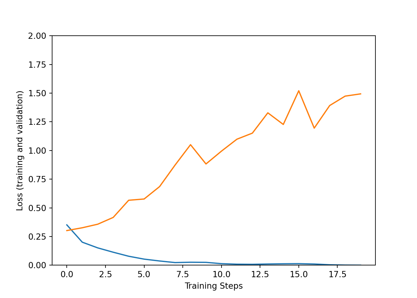
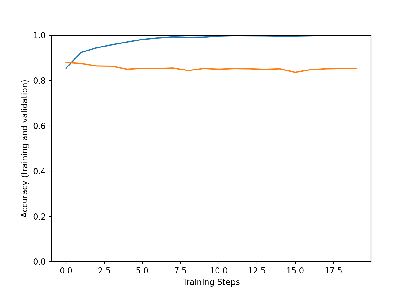
Visualize training process:
"Loss (training and validation)" )"Training Steps" )0 , 2 ])"loss" ])"val_loss" ])"Accuracy (training and validation)" )"Training Steps" )0 , 1 ])"accuracy" ])"val_accuracy" ])
<- 32 cat ('Train... \n ' )system.time ({<- model %>% fit (batch_size = batch_size,epochs = 20 ,validation_data = list (x_test_1h, y_test),verbose = 2
   user  system elapsed
132.116  91.245  58.763
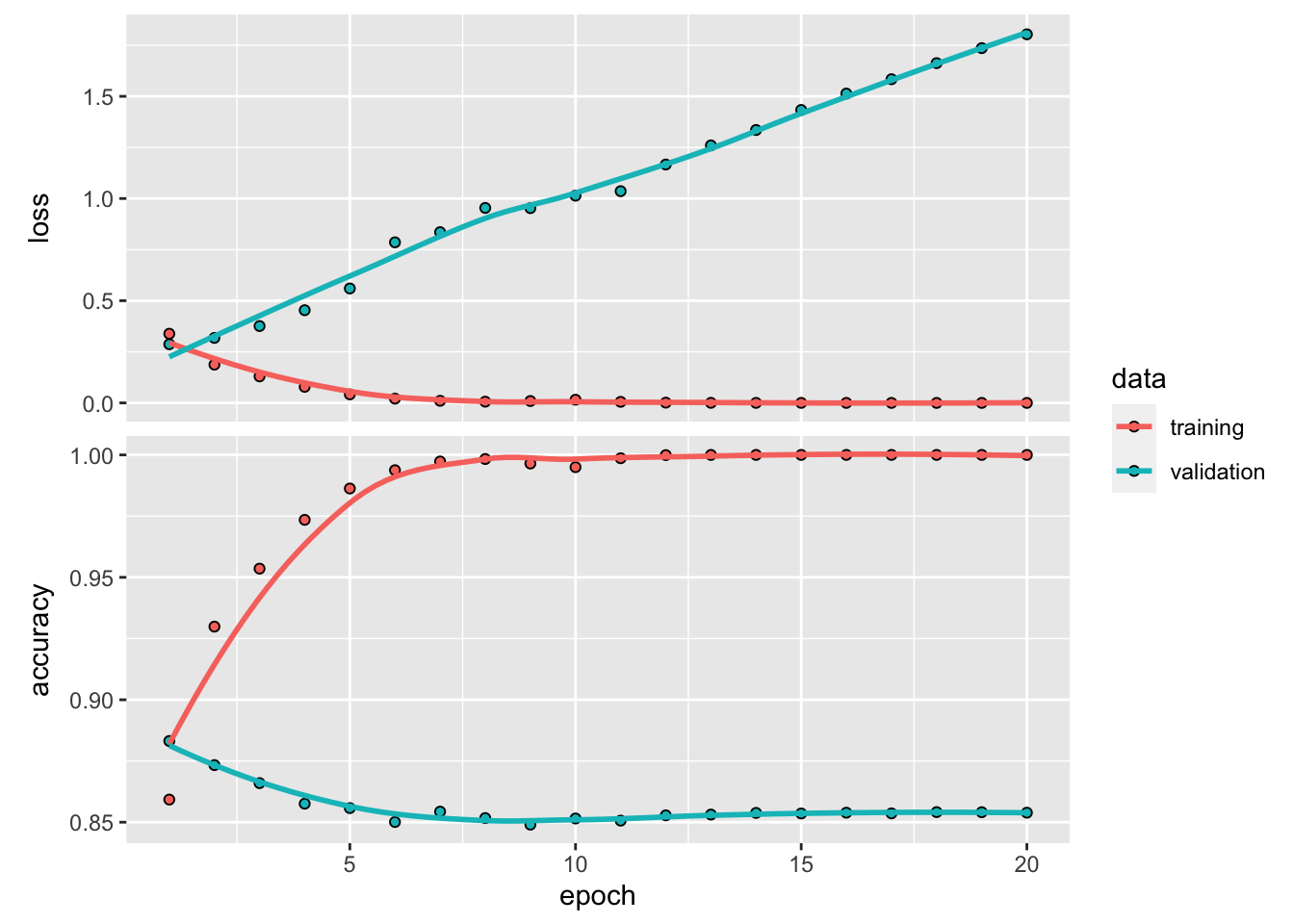
Visualize training process:
Testing
= model.evaluate(= batch_size,= 2
782/782 - 1s - loss: 1.4935 - accuracy: 0.8538 - 767ms/epoch - 981us/step
print ('Test score:' , score)
Test score: 1.4935431480407715
print ('Test accuracy:' , acc)
Test accuracy: 0.8538399934768677
<- model %>% evaluate (batch_size = batch_size
cat ('Test score:' , scores[[1 ]])cat ('Test accuracy' , scores[[2 ]])