Display system information for reproducibility.
import IPythonprint (IPython.sys_info())
{'commit_hash': 'add5877a4',
 'commit_source': 'installation',
 'default_encoding': 'utf-8',
 'ipython_path': '/Users/huazhou/opt/anaconda3/lib/python3.9/site-packages/IPython',
 'ipython_version': '8.8.0',
 'os_name': 'posix',
 'platform': 'macOS-10.16-x86_64-i386-64bit',
 'sys_executable': '/Users/huazhou/opt/anaconda3/bin/python3',
 'sys_platform': 'darwin',
 'sys_version': '3.9.12 (main, Apr  5 2022, 01:56:13) \n[Clang 12.0.0 ]'}
R version 4.2.2 (2022-10-31)
Platform: x86_64-apple-darwin17.0 (64-bit)
Running under: macOS Big Sur ... 10.16

Matrix products: default
BLAS:   /Library/Frameworks/R.framework/Versions/4.2/Resources/lib/libRblas.0.dylib
LAPACK: /Library/Frameworks/R.framework/Versions/4.2/Resources/lib/libRlapack.dylib

locale:
[1] en_US.UTF-8/en_US.UTF-8/en_US.UTF-8/C/en_US.UTF-8/en_US.UTF-8

attached base packages:
[1] stats     graphics  grDevices utils     datasets  methods   base

loaded via a namespace (and not attached):
 [1] Rcpp_1.0.9        here_1.0.1        lattice_0.20-45   png_0.1-8
 [5] withr_2.5.0       rprojroot_2.0.3   digest_0.6.29     grid_4.2.2
 [9] jsonlite_1.8.0    magrittr_2.0.3    evaluate_0.15     rlang_1.0.6
[13] stringi_1.7.8     cli_3.4.1         rstudioapi_0.13   Matrix_1.5-1
[17] reticulate_1.27   rmarkdown_2.14    tools_4.2.2       stringr_1.4.0
[21] htmlwidgets_1.6.1 xfun_0.31         yaml_2.3.5        fastmap_1.1.0
[25] compiler_4.2.2    htmltools_0.5.4   knitr_1.39
Load some libraries.
# Load the pandas library import pandas as pd# Load numpy for array manipulation import numpy as np# Load seaborn plotting library import seaborn as snsimport matplotlib.pyplot as plt# Set font sizes in plots set (font_scale = 1.2 )# Display all columns 'display.max_columns' , None )# Load Tensorflow and Keras import tensorflow as tffrom tensorflow import kerasfrom tensorflow.keras import layers
In this example, we train an MLP (multi-layer perceptron) on the MNIST data set. Achieve testing accuracy 98.11% after 30 epochs.
The MNIST database (Modified National Institute of Standards and Technology database) is a large database of handwritten digits (\(28 \times 28\) ) that is commonly used for training and testing machine learning algorithms.
60,000 training images, 10,000 testing images.
Prepare data
Acquire data:
# Load the data and split it between train and test sets = keras.datasets.mnist.load_data()# Training set
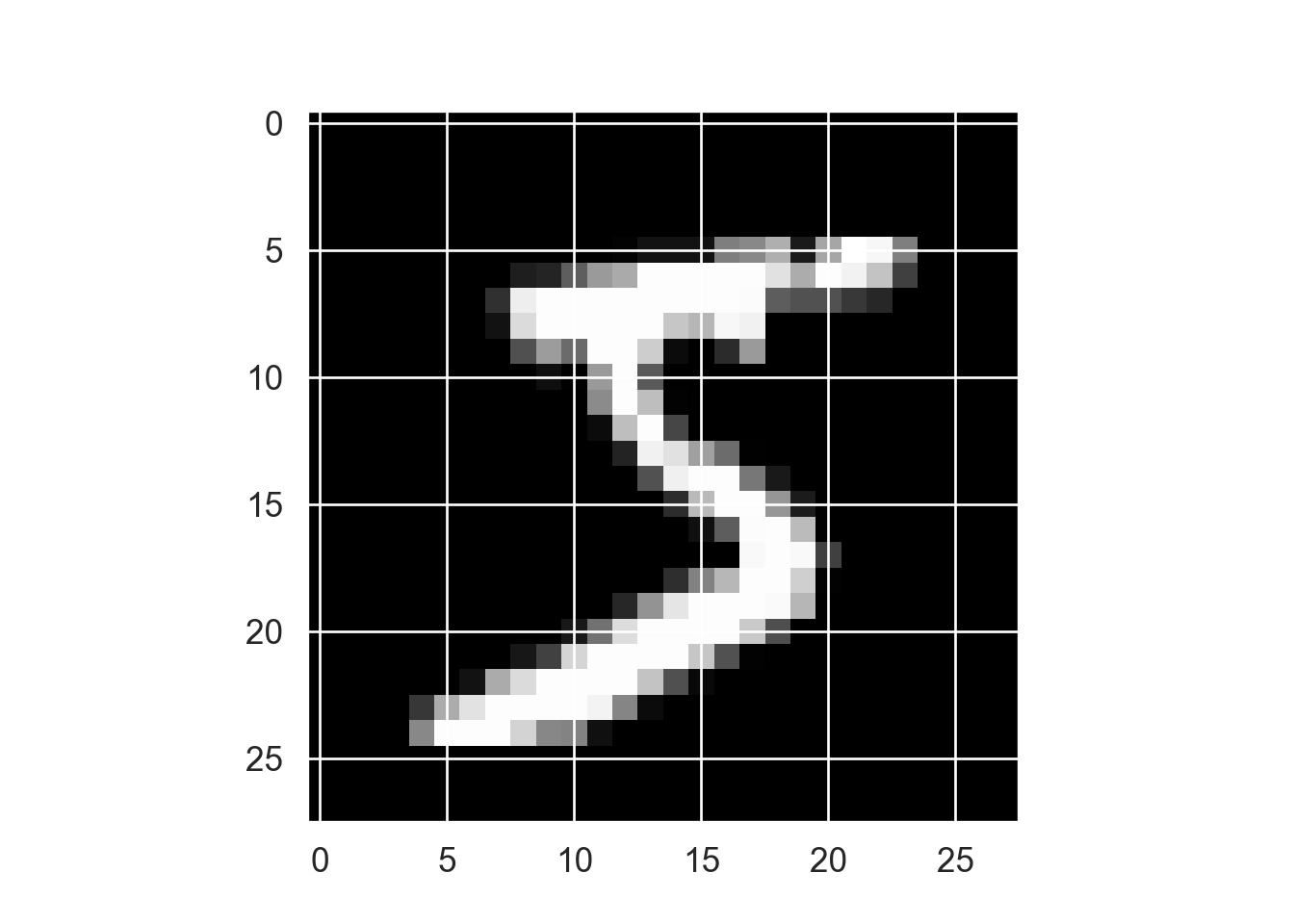
Display the first training instance and its label:
import matplotlib.pyplot as plt# Feature: digit 0 ]); # Label
<- dataset_mnist ()<- mnist$ train$ x<- mnist$ train$ y<- mnist$ test$ x<- mnist$ test$ y
Training set:
image (t (x_train[1 , 28 : 1 ,]), useRaster = TRUE , axes = FALSE , col = grey (seq (0 , 1 , length = 256 ))
Testing set:
Vectorize \(28 \times 28\) images into \(784\) -vectors and scale entries to [0, 1]:
# Reshape = np.reshape(x_train, [x_train.shape[0 ], 784 ])= np.reshape(x_test, [x_test.shape[0 ], 784 ])# Rescale = x_train / 255 = x_test / 255 # Train # Test
# reshape <- array_reshape (x_train, c (nrow (x_train), 784 ))<- array_reshape (x_test, c (nrow (x_test), 784 ))# rescale <- x_train / 255 <- x_test / 255 dim (x_train)
Encode \(y\) as binary class matrix:
= keras.utils.to_categorical(y_train, 10 )= keras.utils.to_categorical(y_test, 10 )# Train # Test # First train instance
array([0., 0., 0., 0., 0., 1., 0., 0., 0., 0.], dtype=float32)
<- to_categorical (y_train, 10 )<- to_categorical (y_test, 10 )dim (y_train)
     [,1] [,2] [,3] [,4] [,5] [,6] [,7] [,8] [,9] [,10]
[1,]    0    0    0    0    0    1    0    0    0     0
[2,]    1    0    0    0    0    0    0    0    0     0
[3,]    0    0    0    0    1    0    0    0    0     0
[4,]    0    1    0    0    0    0    0    0    0     0
[5,]    0    0    0    0    0    0    0    0    0     1
[6,]    0    0    1    0    0    0    0    0    0     0
Define the model
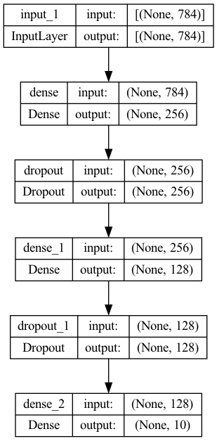
Define a sequential model (a linear stack of layers) with 2 fully-connected hidden layers (256 and 128 neurons):
= keras.Sequential(= (784 ,)),= 256 , activation = 'relu' ),= 0.4 ),= 128 , activation = 'relu' ),= 0.3 ),= 10 , activation = 'softmax' )
Model: "sequential"
_________________________________________________________________
 Layer (type)                Output Shape              Param #
=================================================================
 dense (Dense)               (None, 256)               200960

 dropout (Dropout)           (None, 256)               0

 dense_1 (Dense)             (None, 128)               32896

 dropout_1 (Dropout)         (None, 128)               0

 dense_2 (Dense)             (None, 10)                1290

=================================================================
Total params: 235,146
Trainable params: 235,146
Non-trainable params: 0
_________________________________________________________________
Plot the model:
= "model.png" ,= True ,= False ,= True ,= "TB" ,= False ,= 96 ,= None ,= False ,
<- keras_model_sequential () %>% layer_dense (units = 256 , activation = 'relu' , input_shape = c (784 )) %>% layer_dropout (rate = 0.4 ) %>% layer_dense (units = 128 , activation = 'relu' ) %>% layer_dropout (rate = 0.3 ) %>% layer_dense (units = 10 , activation = 'softmax' )summary (model)
Model: "sequential_1"
________________________________________________________________________________
 Layer (type)                       Output Shape                    Param #
================================================================================
 dense_5 (Dense)                    (None, 256)                     200960
 dropout_3 (Dropout)                (None, 256)                     0
 dense_4 (Dense)                    (None, 128)                     32896
 dropout_2 (Dropout)                (None, 128)                     0
 dense_3 (Dense)                    (None, 10)                      1290
================================================================================
Total params: 235,146
Trainable params: 235,146
Non-trainable params: 0
________________________________________________________________________________
Compile the model with appropriate loss function, optimizer, and metrics:
compile (= "categorical_crossentropy" ,= "rmsprop" ,= ["accuracy" ]
%>% compile (loss = 'categorical_crossentropy' ,optimizer = optimizer_rmsprop (),metrics = c ('accuracy' )
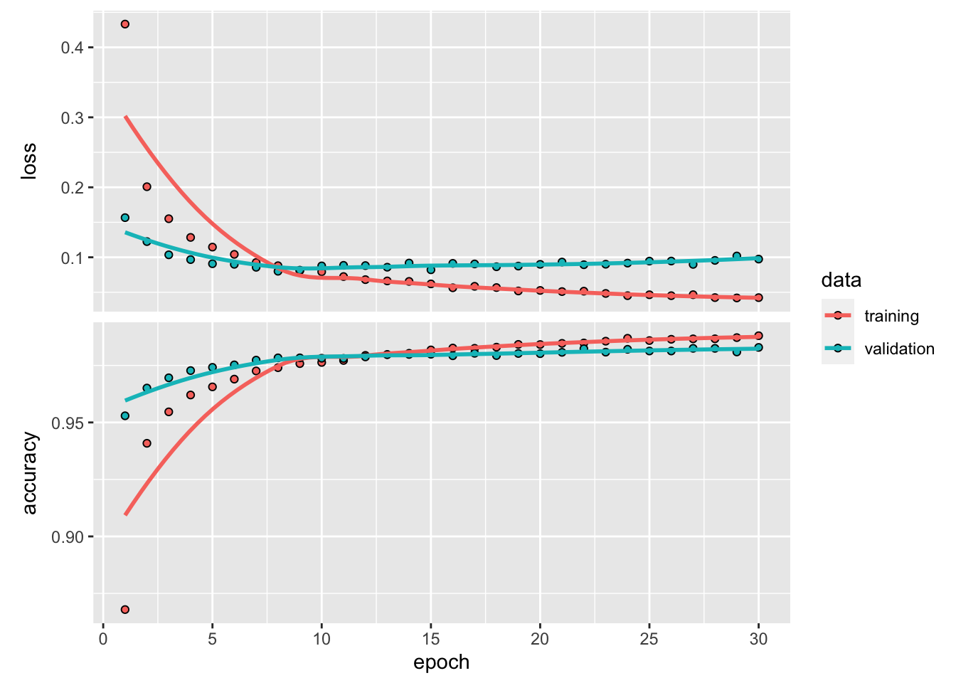
Training and validation
80%/20% split for the train/validation set.
= 128 = 30 = model.fit(= batch_size,= epochs,= 0.2
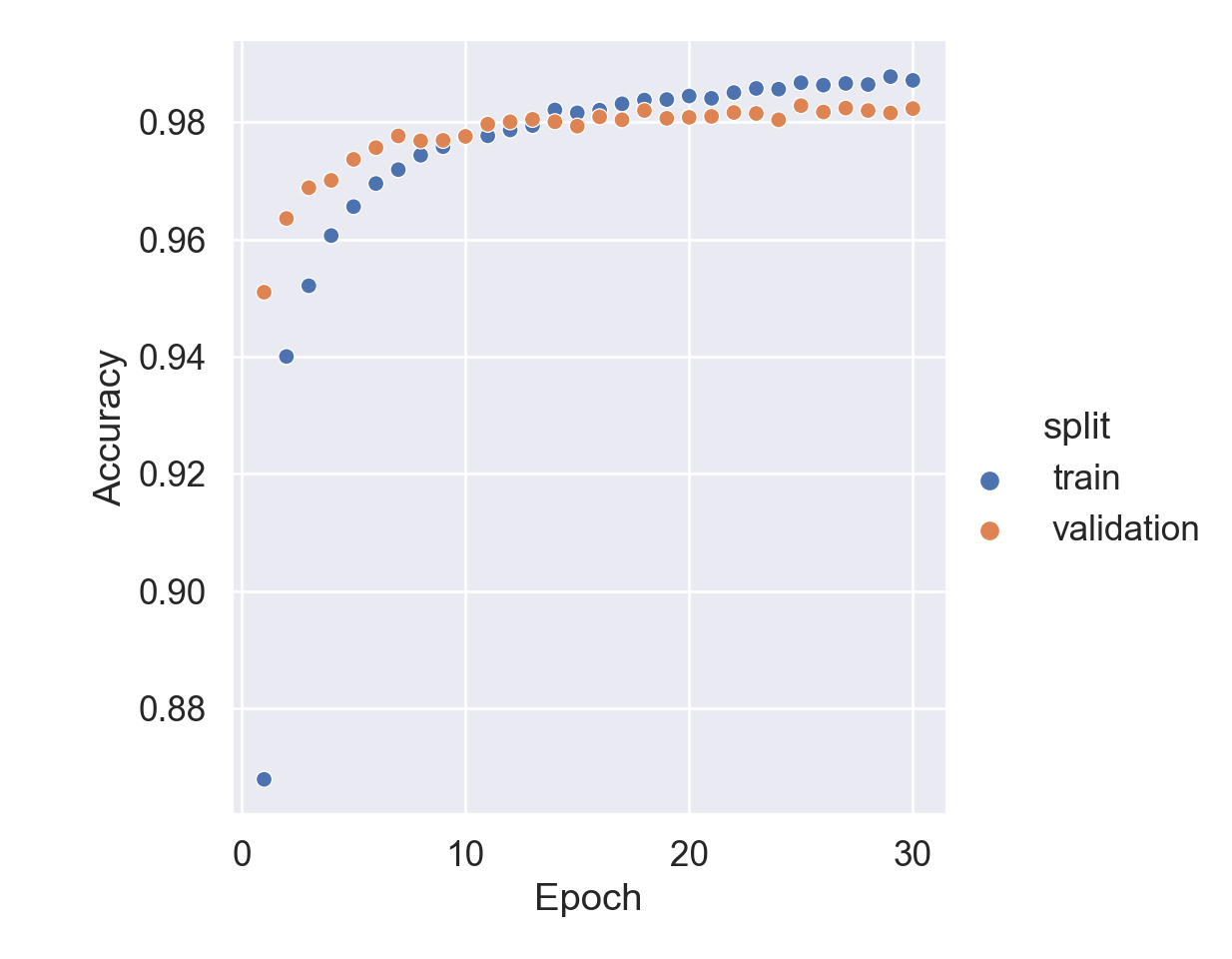
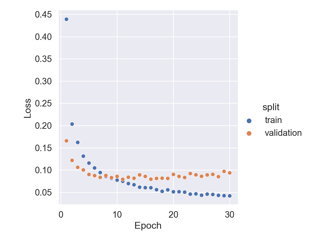
Plot training history:
Code
= pd.DataFrame(history.history)'epoch' ] = np.arange(1 , epochs + 1 )= hist.melt(= ['epoch' ],= ['loss' , 'accuracy' , 'val_loss' , 'val_accuracy' ],= 'type' ,= 'value' 'split' ] = np.where(['val' in s for s in hist['type' ]], 'validation' , 'train' )'metric' ] = np.where(['loss' in s for s in hist['type' ]], 'loss' , 'accuracy' )# Accuracy trace plot = hist[hist['metric' ] == 'accuracy' ],= 'scatter' ,= 'epoch' ,= 'value' ,= 'split' set (= 'Epoch' ,= 'Accuracy' ; # Loss trace plot
Code
= hist[hist['metric' ] == 'loss' ],= 'scatter' ,= 'epoch' ,= 'value' ,= 'split' set (= 'Epoch' ,= 'Loss' ;
system.time ({<- model %>% fit (epochs = 30 , batch_size = 128 , validation_split = 0.2
   user  system elapsed
113.963  38.164  34.649
Testing
Evaluate model performance on the test data:
= model.evaluate(x_test, y_test, verbose = 0 )print ("Test loss:" , score[0 ])
Test loss: 0.08525163680315018
print ("Test accuracy:" , score[1 ])
Test accuracy: 0.9824000000953674
%>% evaluate (x_test, y_test)
      loss   accuracy
0.08609481 0.98229998
Generate predictions on new data:
%>% predict (x_test) %>% k_argmax ()
tf.Tensor([7 2 1 ... 4 5 6], shape=(10000), dtype=int64)
Exercise
Suppose we want to fit a multinomial-logit model and use it as a baseline method to neural networks. How to do that? Of course we can use mlogit or other packages. Instead we can fit the same model using keras, since multinomial-logit is just an MLP with (1) one input layer with linear activation and (2) one output layer with softmax link function.
# set up model library (keras)<- keras_model_sequential () %>% # layer_dense(units = 256, activation = 'linear', input_shape = c(784)) %>% # layer_dropout(rate = 0.4) %>% layer_dense (units = 10 , activation = 'softmax' , input_shape = c (784 ))summary (mlogit)
Model: "sequential_2"
________________________________________________________________________________
 Layer (type)                       Output Shape                    Param #
================================================================================
 dense_6 (Dense)                    (None, 10)                      7850
================================================================================
Total params: 7,850
Trainable params: 7,850
Non-trainable params: 0
________________________________________________________________________________
# compile model %>% compile (loss = 'categorical_crossentropy' ,optimizer = optimizer_rmsprop (),metrics = c ('accuracy' )
Model: "sequential_2"
________________________________________________________________________________
 Layer (type)                       Output Shape                    Param #
================================================================================
 dense_6 (Dense)                    (None, 10)                      7850
================================================================================
Total params: 7,850
Trainable params: 7,850
Non-trainable params: 0
________________________________________________________________________________
# fit model <- mlogit %>% fit (epochs = 20 , batch_size = 128 , validation_split = 0.2
# Evaluate model performance on the test data: %>% evaluate (x_test, y_test)
     loss  accuracy
0.2697336 0.9279000
Generate predictions on new data:
%>% predict (x_test) %>% k_argmax ()
tf.Tensor([7 2 1 ... 4 5 6], shape=(10000), dtype=int64)
Experiment: Change the linear activation to relu in the multinomial-logit model and see the change in classification accuracy.