R version 4.2.2 (2022-10-31)
Platform: x86_64-apple-darwin17.0 (64-bit)
Running under: macOS Big Sur ... 10.16

Matrix products: default
BLAS:   /Library/Frameworks/R.framework/Versions/4.2/Resources/lib/libRblas.0.dylib
LAPACK: /Library/Frameworks/R.framework/Versions/4.2/Resources/lib/libRlapack.dylib

locale:
[1] en_US.UTF-8/en_US.UTF-8/en_US.UTF-8/C/en_US.UTF-8/en_US.UTF-8

attached base packages:
[1] stats     graphics  grDevices utils     datasets  methods   base

loaded via a namespace (and not attached):
 [1] Rcpp_1.0.9        here_1.0.1        lattice_0.20-45   png_0.1-8
 [5] rprojroot_2.0.3   digest_0.6.30     grid_4.2.2        lifecycle_1.0.3
 [9] jsonlite_1.8.4    magrittr_2.0.3    evaluate_0.18     rlang_1.0.6
[13] stringi_1.7.8     cli_3.4.1         rstudioapi_0.14   Matrix_1.5-1
[17] reticulate_1.26   vctrs_0.5.1       rmarkdown_2.18    tools_4.2.2
[21] stringr_1.5.0     glue_1.6.2        htmlwidgets_1.6.0 xfun_0.35
[25] yaml_2.3.6        fastmap_1.1.0     compiler_4.2.2    htmltools_0.5.4
[29] knitr_1.41
usingInteractiveUtilsversioninfo()
1 Overview
In the section we discuss two resampling methods: cross-validation and the bootstrap.
These methods refit a model of interest to samples formed from the training set, in order to obtain additional information about the fitted model.
For example, they provide estimates of test-set prediction error, and the standard deviation and bias of our parameter estimates.
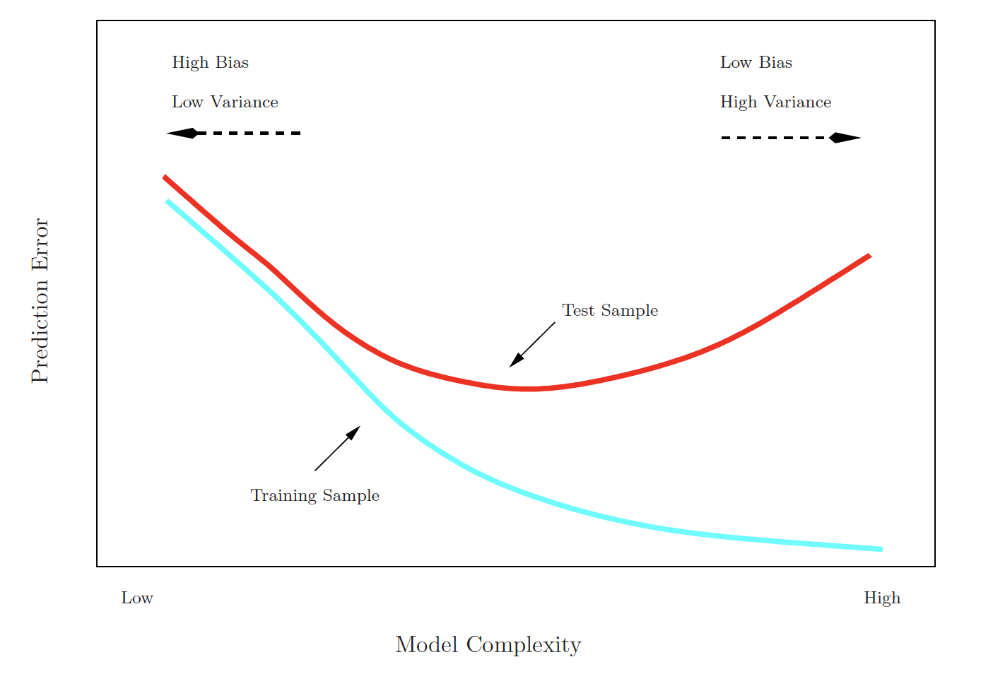
2 Training error vs test error
Test error is the average error that results from using a learning method to predict the response on a new observation, one that was not used in training the method.
Training error can be easily calculated by applying the statistical learning method to the observations used in its training.
But the training error rate often is quite different from the test error rate, and in particular the former can dramatically underestimate the latter.
HW2 Bonus question rigorously justifies that the training error is an under-estimate of the test error.
Best solution: a large designated test set. Often not available.
Some methods make a mathematical adjustment to the training error rate in order to estimate the test error rate. These include the \(C_p\) statistic, AIC and BIC, which are discussed in Chapter 6.
Here we instead consider a class of methods that estimate the test error by holding out a subset of the training observations from the fitting process, and then applying the learning method to those held out observations.
3 Validation-set approach
Here we randomly divide the available set of samples into two parts: a training set and a validation or hold-out set.
The model is fit on the training set, and the fitted model is used to predict the responses for the observations in the validation set.
The resulting validation-set error provides an estimate of the test error. This is typically assessed using MSE in the case of a quantitative response and misclassification rate in the case of a qualitative (discrete) response.
Figure 1: A random splitting into two halves: left part is training set, right part is validation set.
Figure 2: The validation set approach was used on the Auto data set in order to estimate the test error that results from predicting mpg using polynomial functions of horsepower. Left: Validation error estimates for a single split into training and validation data sets. Right: The validation method was repeated ten times, each time using a different random split of the observations into a training set and a validation set. This illustrates the variability in the estimated test MSE that results from this approach.
Drawbacks of validation set approach
The validation estimate of the test error can be highly variable, depending on precisely which observations are included in the training set and which observations are included in the validation set.
In the validation approach, only a subset of the observations - those that are included in the training set rather than in the validation set - are used to fit the model.
This suggests that the validation set error may tend to overestimate the test error for the model fit on the entire data set. (Why?)
4\(K\)-fold cross-validation
Widely used approach for estimating test error.
Estimates can be used to select best model, and to give an idea of the test error of the final chosen model.
Idea is to randomly divide the data into \(K\) equal-sized parts. We leave out part \(k\), fit the model to the other \(K-1\) parts (combined), and then obtain predictions for the left-out \(k\)th part.
This is done in turn for each part \(k = 1, 2, \ldots, K\), and then the results are combined.
Figure 3: A schematic display of 5-fold CV. A set of \(n\) observations is randomly split into five non-overlapping groups. Each of these fifths acts as a validation set (shown in beige), and the remainder as a training set (shown in blue). The test error is estimated by averaging the five resulting MSE estimates.
Let the \(K\) parts be \(C_1, C_2, \ldots, C_K\), where \(C_k\) denotes the indices of the observations in part \(k\). There are \(n_k\) observations in part \(k\). If \(N\) is a multiple of \(K\), then \(n_k = n / K\).
Compute \[
\text{CV}_{(K)} = \sum_{k=1}^K \frac{n_k}{n} \text{MSE}_k,
\] where \[
\text{MSE}_k = \frac{1}{n_k} \sum_{i \in C_k} (y_i - \hat y_i)^2,
\] and \(\hat y_i\) is the fit for observation \(i\), obtained from the data with part \(k\) removed.
4.1 LOOCV
The special case \(K=n\) yields \(n\)-fold or leave-one out cross-validation (LOOCV).
With least-squares linear or polynomial regression, an amazing shortcut makes the cost of LOOCV the same as that of a single model fit! \[
\text{CV}_{(n)} = \frac{1}{n} \sum_{i=1}^n \left( \frac{y_i - \hat y_i}{1 - h_i} \right)^2,
\] where \(\hat y_i\) is the \(i\)th fitted value from the original least squares fit, and \(h_i\) is the leverage (diagonal of the “hat” matrix). This is like the ordinary MSE, except the \(i\)th residual is divided by \(1 - h_i\).
LOOCV sometimes useful, but typically doesn’t shake up the data enough. The estimates from each fold are highly correlated and hence their average can have high variance.
A better choice is \(K = 5\) or 10.
Figure 4: Cross-validation was used on the Auto data set in order to estimate the test error that results from predicting mpg using polynomial functions of horsepower. Left: The LOOCV error curve. Right: 10-fold CV was run nine separate times, each with a different random split of the data into ten parts. The figure shows the nine slightly different CV error curves.
Figure 5: Blue: true test MSE. Black dashed line: LOOCV estimate of test MSE. Orange: 10-fold CV estimate of test MSE. The crosses indicate the minimum of each of the MSE curves. Left data. Middle data. Right data.
5 Bias-variance tradeoff for cross-validation
Since each training set is only \((K - 1) / K\) as big as the original training set, the estimates of prediction error will typically be biased upward. (Why?)
This bias is minimized when \(K = n\) (LOOCV), but this estimate has high variance, as noted earlier.
\(K = 5\) or \(10\) provides a good compromise for this bias-variance trade-off.
6 Cross-validation for classification problems
We divide the data into \(K\) roughly equal-sized parts \(C_1, C_2, \ldots, C_K\). \(C_k\) denotes the indices of the observations in part \(k\). There are \(n_k\) observations in part \(k\). If \(n\) is a multiple of \(K\), then \(n_k = n / K\).
The estimated standard deviation of \(\text{CV}_k\) is \[
\hat{\text{SE}}(\text{CV}_k) = \sqrt{\frac{1}{K} \sum_{k=1}^K \frac{(\text{Err}_k - \bar{\text{Err}_k})^2}{K-1}}.
\] This is a useful estimate, but strictly speaking, not quite valid.
7 Bootstrap
The bootstrap is a flexible and powerful statistical tool that can be used to quantify the uncertainty associated with a given estimator or learning method.
For example, it can provide an estimate of the standard error of a coefficient, or a confidence interval for that coefficient.
A simple example.
Suppose that we wish to invest a fixed sum of money in two financial assets that yield returns of \(X\) and \(Y\), respectively, where \(X\) and \(Y\) are random quantities.
We will invest a fraction \(\alpha\) of our money in \(X\), and will invest the remaining \(1 - \alpha\) in \(Y\).
We wish to choose \(\alpha\) to minimize the total risk, or variance, of our investment. In other words, we want to minimize \(\operatorname{Var}(\alpha X + (1 - \alpha) Y)\).
One can show that the value that minimizes the risk is given by \[
\alpha = \frac{\sigma_{Y}^2 - \sigma_{XY}}{\sigma_X^2 + \sigma_Y^2 - 2 \sigma_{XY}},
\] where \(\sigma_X^2 = \operatorname{Var}(X)\), \(\sigma_Y^2 = \operatorname{Var}(Y)\), and \(\sigma_{XY} = \operatorname{Cov}(X, Y)\).
But the values of \(\sigma_X^2\), \(\sigma_Y^2\), and \(\sigma_{XY}\) are unknown.
We can compute estimates for these quantities \(\hat{\sigma}_X^2\), \(\hat{\sigma}_Y^2\), and \(\hat{\sigma}_{XY}\), using a data set that contains measurements for \(X\) and \(Y\).
We can then estimate the value of \(\alpha\) that minimizes the variance of our investment using \[
\hat{\alpha} = \frac{\hat{\sigma}_{Y}^2 - \hat{\sigma}_{XY}}{\hat{\sigma}_X^2 + \hat{\sigma}_Y^2 - 2 \hat{\sigma}_{XY}}.
\]
Figure 6: Each panel displays 100 simulated returns for investments \(X\) and \(Y\). From left to right and top to bottom, the resulting estimates for \(\alpha\) are 0.576, 0.532, 0.657, and 0.651.
An unrealistic method:
To estimate the standard deviation of \(\hat{\alpha}\), we repeated the process of simulating 100 paired observations of \(X\) and \(Y\), and estimating \(\alpha\) 1,000 times.
We thereby obtained 1,000 estimates for \(\alpha\), which we can call \(\hat{\alpha}_1, \hat{\alpha}_2, \ldots, \hat{\alpha}_{1000}\).
For these simulations the parameters were set to \(\sigma_{X}^2 = 1\), \(\sigma_Y^2 = 1.25\), and \(\sigma_{XY} = 0.5\), and so we know that the true value of \(\alpha\) is 0.6 (indicated by the red line).
The mean over 1,000 estimates for \(\alpha\) is \[
\bar{\alpha} = \frac{1}{1000} \sum_{r=1}^{1000} \hat{\alpha}_r = 0.5996,
\] very close to \(\alpha = 0.6\), and the standard deviation of the estimates is \[
\sqrt{\frac{1}{1000-1} \sum_{r=1}^{1000} (\hat{\alpha}_r - \bar{\alpha})^2} = 0.083.
\] This gives us a very good idea of the accuracy of \(\hat{\alpha}\): \(\text{SE}(\hat{\alpha}) \approx 0.083\). So roughly speaking, for a random sample from the population, we would expect \(\hat{\alpha}\) to differ from \(\alpha\) by approximately 0.08, on average.
Figure 7: A graphical illustration of the bootstrap approach on a small sample containing \(n = 3\) observations. Each bootstrap data set contains \(n\) observations, sampled with replacement from the original data set. Each bootstrap data set is used to obtain an estimate of \(\alpha\).
Bootstrap method.
The procedure outlined above cannot be applied, because for real data we cannot generate new samples from the original population.
However, the bootstrap approach allows us to use a computer to mimic the process of obtaining new data sets, so that we can estimate the variability of our estimate without generating additional samples.
Rather than repeatedly obtaining independent data sets from the population, we instead obtain distinct data sets by repeatedly sampling observations from the original data set with replacement.
Each of these “bootstrap data sets” is created by sampling with replacement, and is the same size as our original dataset. As a result some observations may appear more than once in a given bootstrap data set and some not at all.
Denoting the first bootstrap data set by \(Z^{*1}\), we use \(Z^{*1}\) to produce a new bootstrap estimate for \(\alpha\), which we call \(\hat{\alpha}^{*1}\).
This procedure is repeated \(B\) times for some large value of \(B\) (say 100 or 1000), in order to produce \(B\) different bootstrap data sets \(Z^{*1}, Z^{*2}, \ldots, Z^{*B}\), and \(B\) corresponding \(\alpha\) estimates, \(\hat{\alpha}^{*1}, \hat{\alpha}^{*2}, \ldots, \hat{\alpha}^{*B}\).
We estimate the standard error of these bootstrap estimates using the formula \[
\operatorname{SE}_B(\hat{\alpha}) = \sqrt{\frac{1}{B-1} \sum_{r=1}^B (\hat{\alpha}^{*r} - \bar{\hat{\alpha}}^{*})^2}.
\]
This serves as an estimate of the standard error of \(\hat{\alpha}\) estimated from the original data set. For this example, \(\operatorname{SE}_B(\hat{\alpha}) = 0.087\).
Figure 8: Left: A histogram of the estimates of \(\alpha\) obtained by generating 1,000 simulated data sets from the true population. Center: A histogram of the estimates of \(\alpha\) obtained from 1,000 bootstrap samples from a single data set. Right: The estimates of \(\alpha\) displayed in the left and center panels are shown as boxplots. In each panel, the pink line indicates the true value of \(\alpha\).
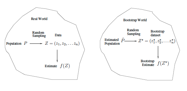
8 Bootstrap in general
Figure 9: Bootstrap general scheme.
In more complex data situations, figuring out the appropriate way to generate bootstrap samples can require some thought.
For example, if the data is a time series (e.g., stock prices), we can’t simply sample the observations with replacement (why not?). We can instead create blocks of consecutive observations, and sample those with replacements. Then we paste together sampled blocks to obtain a bootstrap dataset.
Other uses of the bootstrap.
Primarily used to obtain standard errors of an estimate.
Also provides approximate confidence intervals for a population parameter. For example, looking at the histogram in the middle panel of histogram, the 5% and 95% quantiles of the 1000 values is (0.43, 0.72).
This is called a Bootstrap Percentile confidence interval. It is the simplest method (among many approaches) for obtaining a confidence interval from the bootstrap.
Can the bootstrap estimate prediction error?
In cross-validation, each of the \(K\) validation folds is distinct from the other \(K-1\) folds used for training: there is no overlap. This is crucial for its success.
To estimate prediction error using the bootstrap, we could think about using each bootstrap dataset as our training sample, and the original sample as our validation sample.
But each bootstrap sample has significant overlap with the original data. About two-thirds of the original data points appear in each bootstrap sample. (HW2)
This will cause the bootstrap to seriously underestimate the true prediction error.
The other way around - with original sample = training sample, bootstrap dataset = validation sample - is worse!
Can partly fix this problem by only using predictions for those observations that did not (by chance) occur in the current bootstrap sample.
But the method gets complicated, and in the end, cross-validation provides a simpler, more attractive approach for estimating prediction error.